What is a voice

What makes a voice

Air from the lungs flows up the windpipe and through the larynx, where the two vocal folds sit across the airway. Held together under the right tension, they open and close in a regular cycle, letting air through in puffs: a buzz at the fundamental frequency F_0, the rate of the puffs, with harmonics at every multiple of it. Held apart, the air rushes through as turbulence, a hiss. Either way the larynx is the source. Above it, the throat, mouth and (when the velum is open) the nose form a tube from the larynx to the lips, the vocal tract, which resonates at a few frequencies set by its shape, the formants, and so passes some frequencies of the source more than others. The tract is the filter. At the lips the sound radiates into the air, which favors high frequencies by about 6 dB per octave.

In symbols, the vocal folds open once every period T_0, so the source repeats with the fundamental frequency F_0 = 1/T_0 and its spectrum E(f) has a line at every harmonic kF_0. The tract multiplies it by its gain H(f), and the lips by the radiation R(f):

The source-filter model writes the same product as S = EH, with the radiation folded into the other two. In decibels the product becomes a sum, so the level of harmonic k is the source's level plus the two gains at its frequency:

The tract below is five formants in cascade, each the second-order resonator of Klatt's (1980) synthesizer. For a formant at F_i Hz with bandwidth b_i Hz, sampled at f_s,

with C_i = -e^{-2\pi b_i / f_s}, B_i = 2 e^{-\pi b_i / f_s} \cos(2\pi F_i / f_s) and A_i = 1 - B_i - C_i, which makes the gain 1 at 0 Hz. Each formant is a pair of poles of H at z = e^{-\pi b_i / f_s}\, e^{\pm j 2\pi F_i / f_s}: the angle sets the frequency, and the closer the poles lie to the unit circle, the narrower the bandwidth and the sharper the peak. The lips act as a first difference,

which doubles, that is rises by 6 dB, with every octave well below f_s / 2.

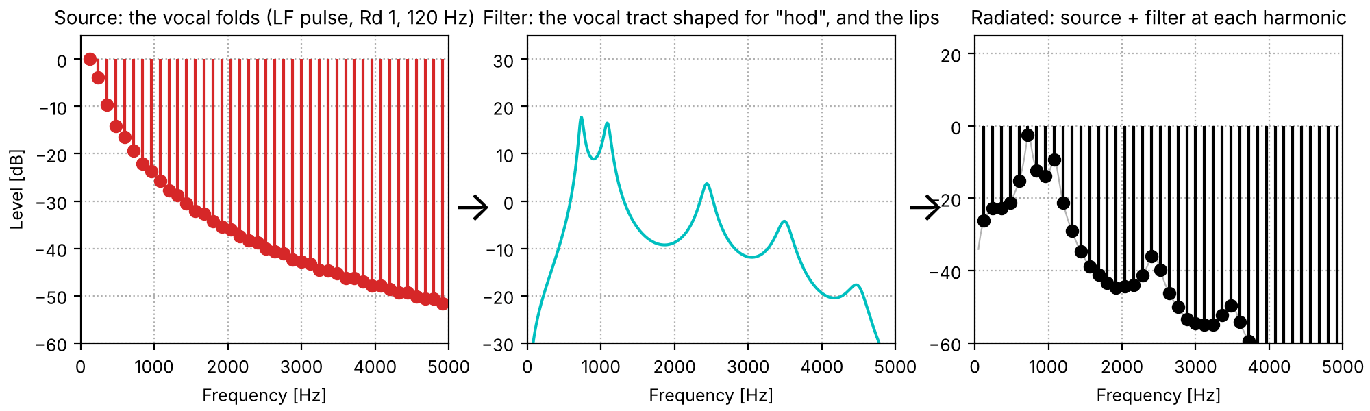
The diagram below draws the chain for one vowel: the harmonics of a glottal pulse, the vocal tract's gain, and their product, which is what reaches a listener. Everything that follows on the voice pages is about measuring the source and the filter from their product, changing one, and putting them back together.

import os
import urllib.request

import matplotlib.pyplot as plt
import numpy as np

import sonore as so

plt.rcParams.update({"font.size": 9, "axes.titlesize": 10, "figure.dpi": 100})


def fetch(path):
    """A file from the sonore repository, by its path there: the local copy when this runs from
    the repository root, otherwise downloaded from GitHub to the same relative path."""
    if not os.path.exists(path):
        os.makedirs(os.path.dirname(path) or ".", exist_ok=True)
        urllib.request.urlretrieve("https://raw.githubusercontent.com/choyun1/sonore/main/" + path, path)
    return path


def finish(snd):
    """How every sound in the gallery is played: 5 ms ramps, RMS 0.1, peak at most 0.95."""
    snd = snd.ramp(5e-3).normalize(rms=0.1)
    return snd.normalize(peak=0.95) if snd.peak > 0.95 else snd

FS = 16000
# The vowel of "hod" as five formants (frequency, bandwidth) in Hz: Peterson and Barney's (1952)
# male and female F1 to F3, with F4 and F5 as on the source-filter page.
HOD = {
    "Male talker": [(730, 60), (1090, 90), (2440, 150), (3500, 200), (4500, 250)],
    "Female talker": [(850, 60), (1220, 90), (2810, 150), (4100, 200), (4900, 250)],
}


def resonator_gain(freq, bandwidth, f):
    """The gain of Klatt's digital resonator at frequencies f (the formula behind so.resonator)."""
    c = -np.exp(-2 * np.pi * bandwidth / FS)
    b = 2 * np.exp(-np.pi * bandwidth / FS) * np.cos(2 * np.pi * freq / FS)
    z = np.exp(-2j * np.pi * f / FS)
    return np.abs((1 - b - c) / (1 - b * z - c * z**2))


def tract_gain_db(f, table):
    return 20 * np.log10(np.prod([resonator_gain(freq, bandwidth, f) for freq, bandwidth in table], axis=0))

Source, filter, and the vowel that reaches a listener

Left: the source, the harmonics of a modal glottal pulse (the LF model at Rd 1) at 120 Hz, whose levels fall off with frequency. Middle: the filter, the gain of the vocal tract shaped for "hod" with the male formants, plus the radiation from the lips. Right: the product, the vowel as it reaches a listener. Each harmonic lands on the source's level plus the filter's gain at its frequency, so the harmonics sample the formants rather than drawing them.

Code

F0_DIAGRAM = 120.0
harmonic_numbers = np.arange(1, int(5000 / F0_DIAGRAM) + 1)
harmonic_freqs = harmonic_numbers * F0_DIAGRAM
source_db = 20 * np.log10(np.abs(so.lf_harmonics(harmonic_numbers, 1.0)))
source_db -= source_db[0]
fine = np.linspace(50, 5000, 2000)
radiation_db = 20 * np.log10(np.abs(1 - np.exp(-2j * np.pi * fine / FS)))
filter_db = tract_gain_db(fine, HOD["Male talker"]) + radiation_db
output_db = source_db + np.interp(harmonic_freqs, fine, filter_db)
fig, axes = plt.subplots(1, 3, figsize=(10, 3.0), layout="constrained")
axes[0].stem(harmonic_freqs, source_db, linefmt="C3-", markerfmt="C3o", basefmt=" ")
axes[0].set(title="Source: the vocal folds (LF pulse, Rd 1, 120 Hz)", ylabel="Level [dB]", ylim=(-60, 5))
axes[1].plot(fine, filter_db, color="c", lw=1.5)
axes[1].set(title='Filter: the vocal tract shaped for "hod", and the lips', ylim=(-30, 35))
axes[2].plot(fine, filter_db + np.interp(fine, harmonic_freqs, source_db), color="0.7", lw=0.8)
axes[2].stem(harmonic_freqs, output_db, linefmt="k-", markerfmt="ko", basefmt=" ")
axes[2].set(title="Radiated: source + filter at each harmonic", ylim=(-60, 25))
for ax in axes:
    ax.set(xlim=(0, 5000), xlabel="Frequency [Hz]")
    ax.grid(ls=":")
for x in (0.345, 0.675):
    fig.text(x, 0.5, "→", fontsize=22, ha="center", va="center")

The two talkers

Every page about speech in this gallery uses one sentence, "Providence had delivered him through the maelstrom," read by two talkers from the CMU ARCTIC corpus (Kominek and Black, 2004): a male talker (speaker bdl) and a female talker (speaker slt), both recorded at 16 kHz. Each analysis is shown on both, because what an analysis gets right on one voice it can get wrong on another, and the most common reason is pitch. Each talker is one person: the numbers on this page describe these two recordings, not men and women in general. Where a page needs averages over many talkers, it cites them.

The code every speech page starts from: the two recordings, each with the pitch track that so.f0_track measures (see Measuring the source: pitch), and a figure with one column per talker.

# The two talkers, by the CMU ARCTIC speaker names. Sources: docs/speech/SOURCES.md.
SPEAKERS = {"Male talker": "bdl", "Female talker": "slt"}
talkers = {
    label: finish(so.load(fetch(f"docs/speech/{speaker}_arctic_a0131.flac")))
    for label, speaker in SPEAKERS.items()
}
tracks = {label: so.f0_track(snd) for label, snd in talkers.items()}


def show_pair(sounds, title, contours=None, fmax=5000):
    """One column per talker: the waveform, and a narrowband spectrogram (Hann 33 ms, which
    resolves the harmonics of both voices) with the pitch track over it if one is given.
    Returns the figure and, for each talker, the panels the playhead follows."""
    fig = plt.figure(figsize=(10, 4.4), layout="constrained")
    columns = fig.subfigures(1, 2)
    playhead = {}
    for column, (label, snd) in zip(columns, sounds.items(), strict=True):
        top, bottom = column.subplots(2, 1, sharex=True, height_ratios=[0.4, 1])
        snd.plot(top, color="k", lw=0.4)
        top.set(title=f"{label}: {title}", xlabel="", ylabel="")
        so.STFT(snd, win_dur=0.0333, hop_dur=0.002).plot(bottom, db_range=70, colorbar=False, fmax=fmax)
        bottom.set_title("Spectrogram (Hann 33 ms)")
        if contours is not None:
            track = contours[label]
            bottom.plot(track.t, np.where(track.voiced[0], track.f0[0], np.nan), color="c", lw=1.2)
        for ax in (top, bottom):
            ax.set_xlim(0, snd.duration)
        playhead[label] = [top, bottom]
    return fig, playhead

The sentence, read by each talker

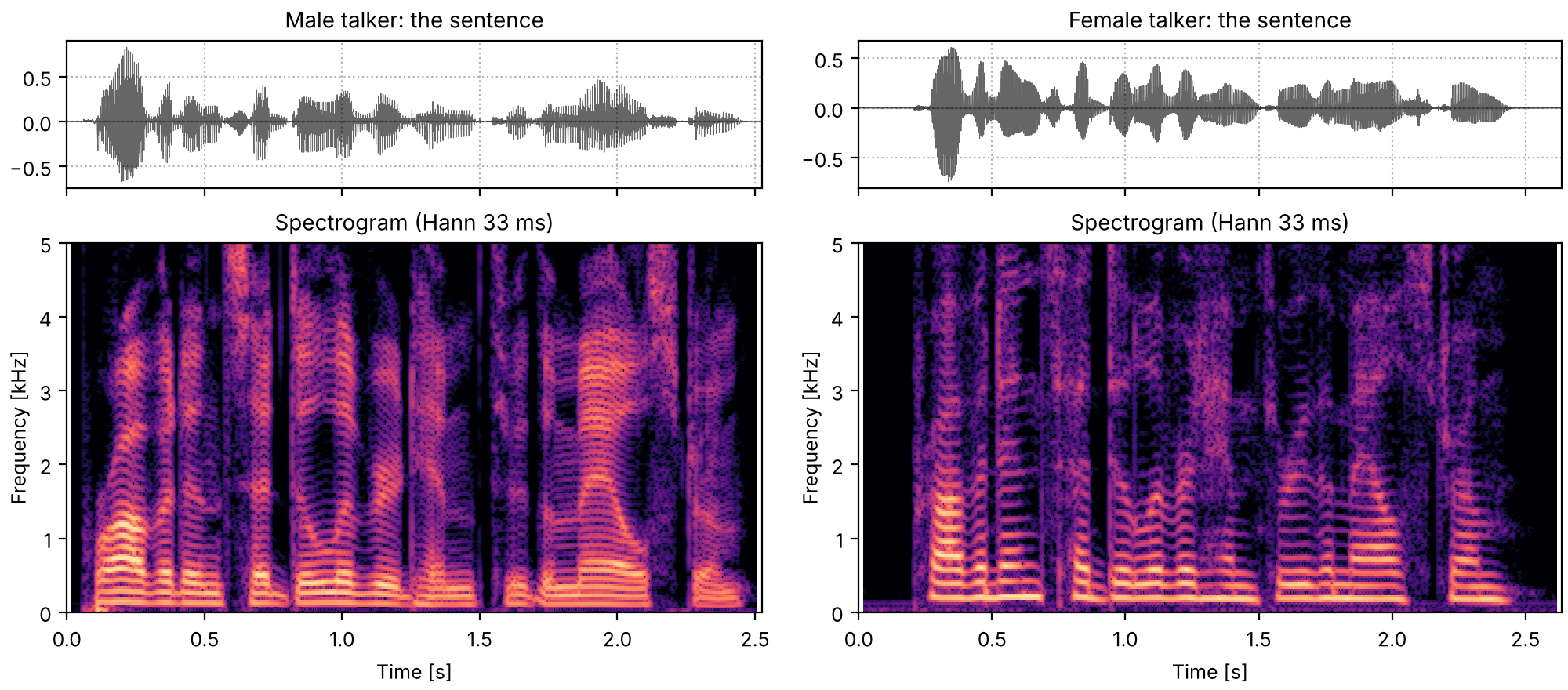
The sentence, read by each talker. The words line up closely: the female talker's reading is 0.1 s longer. The female talker's harmonics, the horizontal lines, are visibly farther apart.

Male talker

tk1_the_sentence_read_by_each_talker_male_talker.flac, 2.5 s, mono

Female talker

tk1_the_sentence_read_by_each_talker_female_talker.flac, 2.6 s, mono

Code

sounds = talkers
fig, playhead = show_pair(sounds, "the sentence")

How voices differ

Two voices saying the same words differ in the source, in the filter, or in both. Each difference below is stated as which of the two it lives in, and how it is measured. Where sonore computes the measure, the page that does so is linked; where it does not, that is said. Clinical voice reports also rate voices by ear, on scales such as GRBAS (Hirano, 1981: grade, roughness, breathiness, asthenia, strain) and CAPE-V (Kempster et al., 2009); the measures below are the acoustic quantities those ratings are usually compared with. This page makes no claim about how its sounds would be rated.

Pitch

In the source. The rate at which the vocal folds open and close, F_0, set by their length, mass and tension; longer and heavier folds vibrate more slowly, which is most of why adult male voices are lower (Titze, 1989). A voice has a level (where F_0 sits), a range (how far it moves) and a variability (how much it moves from moment to moment). Measured from an F0 track, F_0[n] at its N voiced time windows. The interval between two frequencies, in semitones, is

so an octave is 12 semitones and a fifth about 7. The level is the median \tilde F_0. The range is the middle 90%, from the 5th percentile P_5 to the 95th P_{95}, which is \Delta(P_5, P_{95}) semitones wide. The variability is the standard deviation of the track in semitones,

with \bar s the mean of the s_n. The reference \tilde F_0 only sets where zero is, so it does not change \sigma.

voiced_f0 = {label: track.f0[0][track.voiced[0]] for label, track in tracks.items()}
pitch_stats = {}
for label, f0 in voiced_f0.items():
    low, middle, high = np.percentile(f0, [5, 50, 95])
    pitch_stats[label] = dict(median=middle, low=low, high=high, sd=np.std(12 * np.log2(f0 / middle)))
    print(
        f"{label}: median {middle:.0f} Hz, middle 90% {low:.0f} to {high:.0f} Hz "
        f"({12 * np.log2(high / low):.1f} semitones), SD {pitch_stats[label]['sd']:.1f} semitones"
    )
ratio = pitch_stats["Female talker"]["median"] / pitch_stats["Male talker"]["median"]
print(f"female / male median: {ratio:.2f}, {12 * np.log2(ratio):.1f} semitones")

Male talker: median 119 Hz, middle 90% 95 to 144 Hz (7.2 semitones), SD 2.2 semitones
Female talker: median 183 Hz, middle 90% 164 to 210 Hz (4.3 semitones), SD 1.3 semitones
female / male median: 1.53, 7.4 semitones

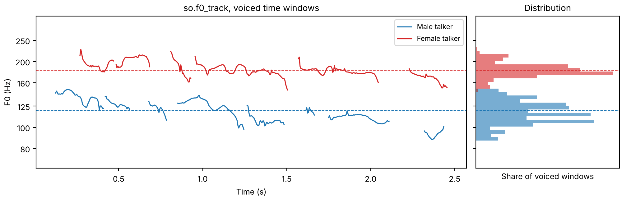
The female talker's voice is about half as high again as the male talker's: a ratio of 1.53, a little more than a fifth (seven semitones, 1.50), and well short of an octave. The male talker's pitch also moves more: 2.2 semitones of standard deviation against 1.3.

The two pitch tracks

Both pitch tracks against time, on a logarithmic frequency axis, where equal intervals are equal distances, and the share of voiced time windows at each pitch. The dashed lines are the medians.

Code

fig, (left, right) = plt.subplots(
    1, 2, figsize=(10, 3.2), layout="constrained", width_ratios=[3, 1], sharey=True
)
bins = np.geomspace(70, 300, 41)
for color, (label, track) in zip(("C0", "C3"), tracks.items(), strict=True):
    left.plot(track.t, np.where(track.voiced[0], track.f0[0], np.nan), color=color, lw=1.2, label=label)
    right.hist(voiced_f0[label], bins=bins, orientation="horizontal", color=color, alpha=0.6, density=True)
    for ax in (left, right):
        ax.axhline(np.median(voiced_f0[label]), color=color, ls="--", lw=0.8)
so.plotting.log_frequency_axis(left)
left.set(xlabel="Time (s)", ylabel="F0 (Hz)", title="so.f0_track, voiced time windows")
left.set_yticks([80, 100, 125, 160, 200, 250], ["80", "100", "125", "160", "200", "250"])
left.set_yticks([], minor=True)
left.legend(loc="upper right", fontsize=8)
right.set(xlabel="Share of voiced windows", title="Distribution")
right.set_xticks([])

Cycle-to-cycle irregularity

In the source. No two glottal cycles are the same length or the same strength. Jitter is the perturbation of the period from one cycle to the next, and shimmer the same for the cycles' peak amplitudes. With T_i the length of the i-th of N consecutive periods and A_i its peak amplitude, the local jitter and shimmer that Praat's voice report gives (Boersma & Weenink, manual pages "Voice 2. Jitter" and "Voice 3. Shimmer") are the mean absolute difference between neighbors over the mean,

usually given in percent, and shimmer is also given in decibels, as the mean of |20 \log_{10}(A_i / A_{i-1})|. Both are read from marks on each individual cycle of the waveform. Clinical reports give them for a sustained vowel, where the voice is meant to be steady. Not in sonore: so.f0_track reads a time window several periods long at a time and cannot see single cycles, so sonore marks no periods and computes neither. What jitter and shimmer do to the analyses here is read as noise (Fit the harmonics, keep the rest).

Noise in the voice

In the source. Turbulence at the glottis adds a hiss to the buzz, which is heard as breathiness; irregular vibration adds a rougher kind of noise, heard as hoarseness. Two measures are common.

The harmonics-to-noise ratio (HNR; Yumoto, Gould & Baer, 1982) is the power of the periodic part over the power of the rest, in dB, which needs the periodic part separated out. Yumoto et al. took n consecutive periods x_i(t), 0 \le t < T_0, of a sustained vowel, called their average \bar x(t) = \frac{1}{n} \sum_i x_i(t) the harmonic part and the differences from it the noise:

A source that is partly noise separates the two frequency by frequency instead, as an aperiodicity: at each time and frequency, the share of the power that is noise, a^2 = P_N / (P_H + P_N) for harmonic power P_H and noise power P_N. Where the share is a^2, the HNR is

so a noise share of -20 dB (1% of the power) is an HNR of about 20 dB.

Cepstral peak prominence (CPP; Hillenbrand, Cleveland & Erickson, 1994) is the height of the cepstrum's pitch peak above the trend of the rest of the cepstrum. With the cepstrum of a time window c(q) = \mathcal{F}^{-1}\{\ln |X(f)|\}(q) (Pitch from the cepstrum) taken in decibels, C(q) = 20 \log_{10} |c(q)|, and \hat C(q) = \alpha q + \beta the straight line fitted to C by least squares,

in dB, the peak searched for among the periods a voice can have. A regular voice with strong harmonics has a tall peak, and noise and irregularity both flatten it. It needs no pitch track, and it is among the acoustic measures clinical studies most often report against ratings of breathiness and overall dysphonia. Both measures are computed in the table below.

Phonation type

In the source. How the vocal folds are held changes the shape of each glottal pulse. Pressed together they close abruptly, and the sharp closure makes strong high harmonics; held loosely they close gradually, leaving little but the fundamental and letting air leak through as noise. Voice scientists describe the range from pressed (or tense, strained) through modal to breathy (lax), and measure it on the source spectrum's tilt: H1–H2, the level of the first harmonic over the second, which rises as the voice gets breathier, and H1–A3, the first harmonic over the strongest harmonic of the third formant (Hanson, 1997). With L(f) the spectrum of a time window in dB and L_k the level of harmonic k, taken as the largest value of L within F_0/4 of kF_0,

with \mathcal{K}_3 the harmonics under the third formant. In the LF model of the glottal pulse the whole shape is one number (Fant, 1995),

with U_0 the peak glottal flow, E_e the strength of the closure (the negative peak of the flow's derivative) and T_0 the period. It runs from about 0.3 (pressed) to 2.7 (breathy), and Fant fitted H1–H2 to it as

Voice quality draws the pulses and their spectra; the vowel below puts three of them on the same vocal tract.

VOWEL_DUR = 1.0
RDS = {0.5: "tense, Rd 0.5", 1.0: "modal, Rd 1", 2.5: "lax, Rd 2.5"}
PITCHES = {"Male talker": ([0, VOWEL_DUR], [130, 100]), "Female talker": ([0, VOWEL_DUR], [230, 200])}


def onoff(dur, level=60, on=0.02, off=0.05):
    """An amplitude track: up over `on` seconds, down over the last `off` seconds."""
    return ([0, on, dur - off, dur], [0, level, level, 0])


def hod_vowels(label):
    """The vowel of "hod" with a talker's formants and pitch, three times with a tense, a modal and
    a lax LF pulse (so.klatt_synthesize's SS=3 source with RD), with a gap between."""
    formants = {f"F{i}": freq for i, (freq, _) in enumerate(HOD[label], start=1)}
    parts = []
    for rd in RDS:
        snd = so.klatt_synthesize(
            VOWEL_DUR, FS, F0=PITCHES[label], AV=onoff(VOWEL_DUR), SS=3, RD=rd, **formants
        )
        parts += [snd, so.silence(0.2, FS)]
    return finish(so.concat(parts[:-1]))

One vowel, three voices

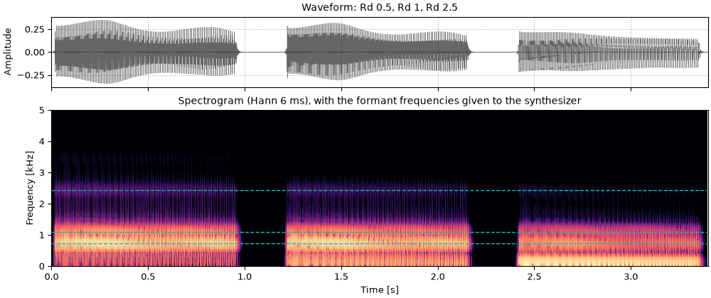
The vowel of "hod" three times, with everything the same except the pulse: tense (Rd 0.5), modal (Rd 1) and lax (Rd 2.5), with the male formants and pitch and with the female ones. The vowel stays the same; the voice goes from pressed and bright to soft and muffled. Since the pulse sets the level of each harmonic by its number, the same Rd at the higher pitch spreads the same levels over a wider range of frequencies. A lax pulse alone sounds soft rather than breathy: Klatt & Klatt (1990) found aspiration noise the most important cue to breathiness, which is why A breathy vowel adds it.

Male talker

fq3_one_vowel_three_voices_male_talker.flac, 3.4 s, mono

Female talker

fq3_one_vowel_three_voices_female_talker.flac, 3.4 s, mono

Code

sounds = {label: hod_vowels(label) for label in talkers}
fig, playhead = show_pair(sounds, "Rd 0.5, 1, 2.5")

Vocal effort

In the source and the filter. A voice raised to be heard over noise or distance is not only louder. The glottal pulses close more sharply, so the spectrum flattens and the high harmonics gain more than the low ones; F_0 rises; the mouth opens wider and the first formant rises with it (Traunmüller & Eriksson, 2000). So effort is read from the spectral tilt, the pitch and F1 together, relative to the same talker speaking normally. The tilt is the slope b, in dB per octave, of the straight line that best fits a spectrum's level L(f) against log frequency over a band \Phi:

A single recording with no quiet or loud counterpart gives no effort measure. Not measured here, for that reason.

Size: the spectral envelopes

In the filter. A longer vocal tract resonates lower. The simplest tract, a uniform tube of length \ell closed at the glottis and open at the lips, resonates where a quarter wavelength, or an odd multiple of one, fits in it (Fant, 1960):

with c \approx 350 m/s the speed of sound in warm, humid air: 500, 1500 and 2500 Hz for a tract 17.5 cm long. Every formant is inversely proportional to the length, so two tracts of the same shape, lengths \ell_1 and \ell_2, have every formant in the same ratio, F_k^{(2)} / F_k^{(1)} = \ell_1 / \ell_2, and the whole spectral envelope slides along a logarithmic frequency axis by \log(\ell_1 / \ell_2) without changing shape. Real tracts are not uniform, so this holds to a first approximation (Fitch & Giedd, 1999). Adult men have tracts about 15 to 20% longer than adult women's, and children's are shorter again, which is why a child's vowels sit higher even at the same pitch. Measured two ways here: as the ratio that best moves one talker's average spectral envelope onto the other's, and in the table below as the ratio of their median formant frequencies.

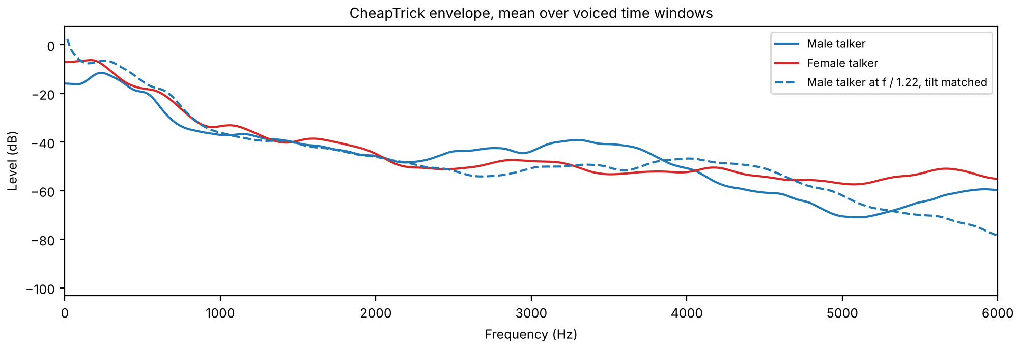
The formants are the peaks of the spectral envelope, the shape the vocal tract gives the harmonics. CheapTrick's envelope (Morise, 2015; An envelope measured to the pitch period) is measured every 5 ms, as a power P(t, f); averaging it in dB over each talker's voiced time windows V gives one curve per talker,

The cell reads the male average at f/r and finds the r that brings it closest to the female one over the bins \Phi from 100 to 5000 Hz, in RMS dB, with the level a and the tilt b left free:

and again with only the level free (b = 0).

envelopes = {label: so.pitch_adaptive_envelope(talkers[label], tracks[label]) for label in talkers}
frequencies = envelopes["Male talker"].f
scored = (frequencies >= 100) & (frequencies <= 5000)
average_db = {
    label: np.mean(10 * np.log10(env(tracks[label].t[tracks[label].voiced[0]], frequencies)[0]), axis=1)
    for label, env in envelopes.items()
}


def misfit(ratio, tilt=False):
    """RMS dB between the female average and the male one read at f / ratio, 100 to 5000 Hz,
    with the level (and, if tilt is True, a tilt) left free."""
    male_read = np.interp(frequencies[scored] / ratio, frequencies, average_db["Male talker"])
    difference = average_db["Female talker"][scored] - male_read
    columns = [np.ones(scored.sum())] + ([np.log2(frequencies[scored])] if tilt else [])
    basis = np.column_stack(columns)
    return np.sqrt(np.mean((difference - basis @ np.linalg.lstsq(basis, difference, rcond=None)[0]) ** 2))


ratios = np.arange(0.80, 2.00, 0.005)
for tilt in (False, True):
    errors = [misfit(r, tilt) for r in ratios]
    best = ratios[np.argmin(errors)]
    print(f"{'level and tilt free' if tilt else 'level free':20}: r = {best:.3f}, {min(errors):.2f} dB RMS")
warp = ratios[np.argmin([misfit(r, True) for r in ratios])]

level free          : r = 1.645, 4.34 dB RMS
level and tilt free : r = 1.220, 2.89 dB RMS

With only the level free, the best ratio is large, because the female talker's average envelope is also tilted differently, and moving formants is the only thing the fit can do about it. With the tilt free too, the ratio falls to 1.22. Changing a voice toward the other (Rebuilding and changing a voice) has to move the formants and the tilt separately: size and phonation type are two differences, not one.

The two average envelopes

The two average envelopes, and the male one read at f / r with the r just fitted with the tilt free, its level and tilt then matched to the female one over 100 to 5000 Hz.

Code

fig, ax = plt.subplots(figsize=(10, 3.4), layout="constrained")
male_read = np.interp(frequencies / warp, frequencies, average_db["Male talker"])
basis = np.column_stack([np.ones(scored.sum()), np.log2(frequencies[scored])])
level, tilt = np.linalg.lstsq(basis, average_db["Female talker"][scored] - male_read[scored], rcond=None)[0]
male_level = np.mean(average_db["Female talker"][scored] - average_db["Male talker"][scored])
ax.plot(frequencies, average_db["Male talker"] + male_level, color="C0", label="Male talker")
ax.plot(frequencies, average_db["Female talker"], color="C3", label="Female talker")
ax.plot(
    frequencies[1:],
    male_read[1:] + level + tilt * np.log2(frequencies[1:]),
    color="C0",
    ls="--",
    label=f"Male talker at f / {warp:.2f}, tilt matched",
)
ax.set(xlabel="Frequency (Hz)", ylabel="Level (dB)", xlim=(0, 6000))
ax.set_title("CheapTrick envelope, mean over voiced time windows")
ax.legend(loc="upper right", fontsize=8)

A few indicators, measured

Of the measures above, sonore already computes the parts that these five need, so the cell measures them on both recordings. Each is defined in the code, over the voiced time windows of the so.f0_track track, and each leaves something out:

• F0: the median \tilde F_0 and the middle 90% range, P_5 to P_{95}, from above.
• H1–H2: L_1 - L_2 as defined above, in each 40 ms Hann time window; the median over time windows. Uncorrected for the vocal tract: a first formant near either harmonic raises it (Hanson, 1997, corrects for that), so on running speech this is the raw difference, not the source's.
• CPP: C(q^*) - \hat C(q^*) as defined above, from so.Cepstrum of the same time windows, with the line \hat C fitted from 1 ms up to half the window and the peak searched for from 2.5 to 16.7 ms (F_{\min} = 60 Hz, F_{\max} = 400 Hz); the median over time windows. Hillenbrand et al. (1994) defined it on the cepstrum of the log power spectrum of a sustained vowel, so these values compare the two talkers with each other, not with clinical software's.
• Noise share: the share a^2(t, f) from so.harmonic_aperiodicity, averaged over each of four bands B with the envelope's power as weight, \sum_{f \in B} a^2 P \big/ \sum_{f \in B} P, which is the band's noise power over its total power; the median over time windows, in dB (0 dB is all noise). Jitter and shimmer count as noise here; D4C's measure, which What D4C reports explains, would give different numbers below 3 kHz.
• Formant scaling: so.formant_track's median F1, F2 and F3 (ceiling 5000 Hz for the male talker, 5500 Hz for the female one, as Praat advises), their ratios, and the geometric mean of the three, s = \bigl(\prod_{k=1}^{3} \tilde F_k^{\mathrm{F}} / \tilde F_k^{\mathrm{M}}\bigr)^{1/3}, to set beside the envelope warp above. In the uniform tube, s is the ratio of the tract lengths, \ell_{\mathrm{M}} / \ell_{\mathrm{F}}.

band_edges = [0, 1000, 2000, 4000, 8000]
CEILINGS = {"Male talker": 5000, "Female talker": 5500}
indicators = {}
for label, snd in talkers.items():
    track = tracks[label]
    stft = so.STFT(snd, win_dur=0.040, hop_dur=0.005)
    cepstrum = so.Cepstrum(stft)
    voiced = np.interp(stft.t, track.t, track.voiced[0].astype(float)) > 0.5
    f0_at = np.interp(stft.t, track.t, track.f0[0])
    magnitude_db = 20 * np.log10(np.abs(stft.data[0]) + 1e-12)

    # The largest spectral peak within F0 / 4 of each harmonic, per voiced time window.
    harmonic_levels = [
        np.array(
            [
                magnitude_db[np.abs(stft.f - number * f0_at[j]) < f0_at[j] / 4, j].max()
                for j in np.nonzero(voiced)[0]
            ]
        )
        for number in (1, 2)
    ]
    h1_h2 = harmonic_levels[0] - harmonic_levels[1]

    quefrency = cepstrum.q
    pitch_range = (quefrency >= 1 / 400) & (quefrency <= 1 / 60)
    trend_range = (quefrency >= 1e-3) & (quefrency <= quefrency.max() / 2)
    cpp = []
    for j in np.nonzero(voiced)[0]:
        cepstrum_db = 20 * np.log10(np.abs(cepstrum.data[0][:, j]) + 1e-12)
        slope, intercept = np.polyfit(quefrency[trend_range], cepstrum_db[trend_range], 1)
        peak = np.argmax(np.where(pitch_range, cepstrum_db, -np.inf))
        cpp.append(cepstrum_db[peak] - (slope * quefrency[peak] + intercept))

    aperiodicity = so.harmonic_aperiodicity(snd, track)
    voiced_windows = np.interp(aperiodicity.t, track.t, track.voiced[0].astype(float)) > 0.5
    shares = aperiodicity.bands(band_edges, envelope=envelopes[label])[0][:, voiced_windows]

    formant_tracks = so.formant_track(snd, ceiling=CEILINGS[label])
    voiced_formants = np.interp(formant_tracks.t, track.t, track.voiced[0].astype(float)) > 0.5
    formants = np.nanmedian(formant_tracks.frequencies[0][:, voiced_formants], axis=1)

    indicators[label] = dict(
        h1_h2=np.median(h1_h2),
        cpp=np.median(cpp),
        shares=10 * np.log10(np.median(shares, axis=1)),
        formants=formants,
    )

bands = "".join(f"{f'{low}-{high}':>10}" for low, high in zip(band_edges[:-1], band_edges[1:], strict=True))
print(f"{'':<30}{'Male talker':>14}{'Female talker':>16}")
for name, key, fmt in (("F0 median [Hz]", "median", ".0f"), ("F0 middle 90% [Hz]", None, None)):
    if key:
        print(
            f"{name:<30}"
            + "".join(f"{pitch_stats[label][key]:>{14 + 2 * i}{fmt}}" for i, label in enumerate(talkers))
        )
    else:
        print(
            f"{name:<30}"
            + "".join(
                f"{pitch_stats[label]['low']:.0f} to {pitch_stats[label]['high']:.0f}".rjust(14 + 2 * i)
                for i, label in enumerate(talkers)
            )
        )
for name, key in (("H1-H2 [dB]", "h1_h2"), ("CPP [dB]", "cpp")):
    print(
        f"{name:<30}"
        + "".join(f"{indicators[label][key]:>{14 + 2 * i}.1f}" for i, label in enumerate(talkers))
    )
print(f"{'Noise share [dB], band [Hz]':<30}{bands}")
for label in talkers:
    print(f"{'  ' + label:<30}" + "".join(f"{value:>10.1f}" for value in indicators[label]["shares"]))
print(
    f"{'Median F1, F2, F3 [Hz]':<30}"
    + "".join(
        f"{', '.join(f'{f:.0f}' for f in indicators[label]['formants']):>{14 + 2 * i}}"
        for i, label in enumerate(talkers)
    )
)
formant_ratios = indicators["Female talker"]["formants"] / indicators["Male talker"]["formants"]
scaling = float(np.exp(np.mean(np.log(formant_ratios))))
ratios_text = ", ".join(f"{r:.2f}" for r in formant_ratios)
print(f"{'Female / male formants':<30}{ratios_text:>14}  geometric mean {scaling:.2f}")
h1_h2_difference = indicators["Female talker"]["h1_h2"] - indicators["Male talker"]["h1_h2"]

                                 Male talker   Female talker
F0 median [Hz]                           119             183
F0 middle 90% [Hz]                 95 to 144      164 to 210
H1-H2 [dB]                              -4.2             8.0
CPP [dB]                                22.8            21.9
Noise share [dB], band [Hz]       0-1000 1000-2000 2000-4000 4000-8000
  Male talker                      -21.3      -7.9      -2.4      -1.1
  Female talker                    -28.7     -10.8      -3.5      -1.6
Median F1, F2, F3 [Hz]        385, 1388, 2643 490, 1677, 2996
Female / male formants        1.27, 1.21, 1.13  geometric mean 1.20

Two of the five tell the two talkers apart, and three do not. The pitch does, as above. The formants scale by 1.20 on the median tracks, close to the 1.22 that moved the whole envelope. In the first approximation that is a male tract 20% longer than the female one, or a female tract 17% shorter, within the range the literature gives for adult men against adult women. H1–H2 differs by 12 dB in the direction of a breathier female voice, but uncorrected for the vocal tract that number is not the source's alone. The CPPs are within a decibel of each other, and the noise shares within a few decibels in every band: by these measures the two recordings are equally regular and equally clean, which is what two unremarkable voices reading a sentence should show.

What this page leaves out

• Jitter, shimmer and HNR as clinical software reports them. They need period marks, which sonore does not make, and a sustained vowel, which the recordings do not contain.
• A corrected H1–H2. The correction for the first formant's boost (Hanson, 1997; Iseli, Shue & Alwan, 2007) needs F1 and its bandwidth in each time window.
• Vocal effort, which needs the same talker at two levels.
• Vocal tract length itself. The formant ratio is its first approximation; the tract is a tube of varying shape, and the formants of a vowel depend on that shape as much as on length.
• The anatomy. The diagram is of spectra, not of the larynx and tract; the folds' tissue layers, the registers (modal, falsetto, fry) and the nasal branch are named nowhere here.
• Children's voices, and anyone but these two talkers.

References

• Boersma & Weenink. Praat: doing phonetics by computer (computer program). Manual pages Voice 2. Jitter and Voice 3. Shimmer. Local jitter and shimmer.
• Fant (1960). Acoustic Theory of Speech Production. Mouton, The Hague. The quarter-wave tube.
• Fant (1995). The LF-model revisited. Transformations and frequency domain analysis. STL-QPSR 36(2–3), 119–156. The Rd parameter and its fit to H1–H2. waveforms.glottal_source
• Fitch & Giedd (1999). Morphology and development of the human vocal tract: a study using magnetic resonance imaging. J. Acoust. Soc. Am. 106(3), 1511–1522. doi:10.1121/1.427148.
• Hanson (1997). Glottal characteristics of female speakers: acoustic correlates. J. Acoust. Soc. Am. 101(1), 466–481. doi:10.1121/1.417991. H1–H2 and H1–A3, and their correction for the formants.
• Hillenbrand, Cleveland & Erickson (1994). Acoustic correlates of breathy vocal quality. J. Speech Hear. Res. 37(4), 769–778. doi:10.1044/jshr.3704.769. Cepstral peak prominence.
• Hirano (1981). Clinical Examination of Voice. Springer. The GRBAS scale.
• Iseli, Shue & Alwan (2007). Age, sex, and vowel dependencies of acoustic measures related to the voice source. J. Acoust. Soc. Am. 121(4), 2283–2295. doi:10.1121/1.2697522.
• Kempster, Gerratt, Verdolini Abbott, Barkmeier-Kraemer & Hillman (2009). Consensus auditory-perceptual evaluation of voice: development of a standardized clinical protocol. Am. J. Speech-Lang. Pathol. 18(2), 124–132. doi:10.1044/1058-0360(2008/08-0017). CAPE-V.
• Klatt (1980). Software for a cascade/parallel formant synthesizer. J. Acoust. Soc. Am. 67(3), 971–995. doi:10.1121/1.383940. The resonator.
• Klatt & Klatt (1990). Analysis, synthesis, and perception of voice quality variations among female and male talkers. J. Acoust. Soc. Am. 87(2), 820–857. doi:10.1121/1.398894. klatt.klatt_synthesize
• Kominek & Black (2004). The CMU Arctic speech databases. Proc. 5th ISCA Speech Synthesis Workshop, 223–224. ISCA Archive. The sentence, by speakers bdl and slt.
• Morise (2015). CheapTrick, a spectral envelope estimator for high-quality speech synthesis. Speech Communication 67, 1–7. doi:10.1016/j.specom.2014.09.003. spectral_envelope.pitch_adaptive_envelope
• Peterson & Barney (1952). Control methods used in a study of the vowels. J. Acoust. Soc. Am. 24(2), 175–184. ASA. The formants of "hod".
• Titze (1989). Physiologic and acoustic differences between male and female voices. J. Acoust. Soc. Am. 85(4), 1699–1707. doi:10.1121/1.397959.
• Traunmüller & Eriksson (2000). Acoustic effects of variation in vocal effort by men, women, and children. J. Acoust. Soc. Am. 107(6), 3438–3451. doi:10.1121/1.429414.
• Yumoto, Gould & Baer (1982). Harmonics-to-noise ratio as an index of the degree of hoarseness. J. Acoust. Soc. Am. 71(6), 1544–1550. doi:10.1121/1.387808.