A spectrogram shows how a sound's power spectrum changes over time. A modulation
spectrogram does the same for its modulation spectrum: how fast, and how deeply, the
envelope of each frequency band rises and falls, moment by moment (Greenberg & Kingsbury,
1997; Kingsbury et al., 1998). It has three axes, time, acoustic frequency and modulation
rate, so it is a cube, and a page can only show cuts through it. Here every example has two:
modulation rate against time, pooled over the acoustic bands, beside the plot; and acoustic
frequency against modulation rate at the current moment (Atlas & Shamma, 2003), which changes
as the sound plays.
How it is computed: band envelopes, then a bank of windowed complex exponentials on each envelope.
Press play and a line follows the sound across every time axis in its plots. Click any time
axis to play from that point. Start with your volume low.
How it is computed
The sound first goes through 24 ERB-spaced bands from 100 Hz to 7 kHz, and each band's
envelope is taken at 1000 Hz (a cochleagram). Each envelope then goes through a bank of
modulation filters, one per rate from 0.5 to 64 Hz. A filter is a complex exponential at its
rate under a Hann window, so it measures the envelope's Fourier component at that rate over
the window, the way one bin of an STFT does for the sound itself. The same window, without
the exponential, measures the envelope's local mean, and the ratio of the two is the
modulation depth:
m_{b,k}(t) = \frac{2\,|y_{b,k}(t)|}{\mu_{b,k}(t)}
A band whose envelope is 1 + m \sin(2\pi f_m t) reads m at the rate f_m, so 100%
modulation is 0 dB and 50% is -6 dB. Depth says how modulated a band is, whatever its
level, which is what makes a quiet band's rhythm as visible as a loud one's.
The window sets the trade-off, as in an STFT. By default each rate's window holds three of
its cycles: 6 s at 0.5 Hz, 0.75 s at 4 Hz, 47 ms at 64 Hz, so slow rates are resolved finely
and fast rates are placed precisely in time. Rates are half an octave apart. A window of six
cycles, with rates a quarter-octave apart, separates rates twice as finely and follows changes
half as quickly; the examples show both. Cells drawn grey are ones the analysis cannot trust:
where the window runs past either end of the sound, or where the rate is faster than the band
is wide (a band's envelope can't change faster than that).
The image beside each player is the default analysis at one moment, band by band. It is
noisier than the pooled plots. The envelope of a narrow band of noise fluctuates at random,
so even steady noise has some depth at every rate, more at fast rates (about -35 dB at
0.5 Hz, -12 dB at 64 Hz). In one band that depth scatters by about 5 dB from moment to
moment; pooled over the 24 bands it scatters by less than 1 dB. Press play,
or click a time axis, and it follows the sound; before that it shows a moment chosen for each
example.
Code
import matplotlib.pyplot as plt
import numpy as np

import sonore as so

plt.rcParams.update({"font.size": 9, "axes.titlesize": 10, "figure.dpi": 100})
fs = 16000
rng = np.random.default_rng(0)


def finish(snd):
    """How every sound in the gallery is played: 5 ms ramps, RMS 0.1, peak at most 0.95."""
    snd = snd.ramp(5e-3).normalize(rms=0.1)
    return snd.normalize(peak=0.95) if snd.peak > 0.95 else snd


def analyze(snd):
    """The cochleagram, and modulation spectrograms with 3-cycle (default) and 6-cycle windows."""
    env = so.cosine_filterbank(n_bands=24, f_lo=100, f_hi=7000).analyze(snd).envelopes(fs=1000)
    return env, so.ModulationSpectrogram(env), so.ModulationSpectrogram(env, cycles=6, per_octave=4)


def show(snd, marks=(), start=None):
    """The cochleagram and both modulation spectrograms, one above the other, with dashed lines
    at ``marks`` [s]; and the band x rate depth image (3 cycles) that follows the sound."""
    env, msg, fine = analyze(snd)
    fig, axes = plt.subplots(3, 1, figsize=(9, 8.4), layout="constrained", sharex=True)
    env.plot(ax=axes[0])
    axes[0].set(title="Cochleagram", xlabel="")
    msg.plot(ax=axes[1])
    axes[1].set(title="Modulation spectrogram, 3 cycles, half-octave rates (pooled over bands)", xlabel="")
    fine.plot(ax=axes[2])
    axes[2].set_title("Modulation spectrogram, 6 cycles, quarter-octave rates (pooled over bands)")
    for ax in axes:
        for m in marks:
            ax.axvline(m, color="c", lw=1, ls="--")
    db = 20 * np.log10(msg.depth[0])
    db[~msg.valid] = np.nan
    top = np.nanmax(db)
    live = {
        "t": msg.t,
        "image": db,
        "x": msg.fm,
        "y": msg.f,
        "range": (top - 30, top),
        "xlabel": "Modulation rate [Hz]",
        "ylabel": "Frequency [Hz]",
        "title": "Depth",
        "start": snd.duration / 2 if start is None else start,
    }
    return fig, list(axes), live
A modulation rate that glides
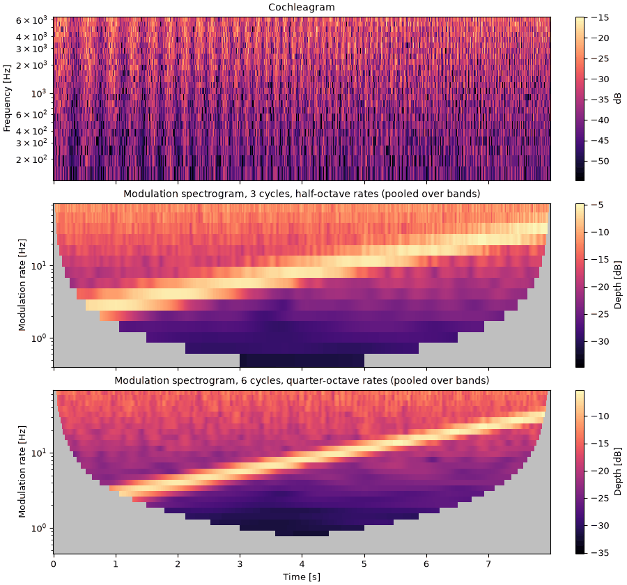
Noise whose amplitude is modulated at a rate that rises smoothly from 2 to 32 Hz over 8 s,
at 50% depth throughout. The modulation is applied to the whole noise, so every band carries
it.
A gliding modulation rate
You hear a slow throb speed up into a flutter and then a rough buzz. The cochleagram is a
blur of noise, but both modulation spectrograms show one line climbing four octaves. The
6-cycle line is thinner, since its windows are longer; the 3-cycle line follows the start more
closely. Next to the player, every band lights up at the same rate at once: the modulation is
common to all frequencies.
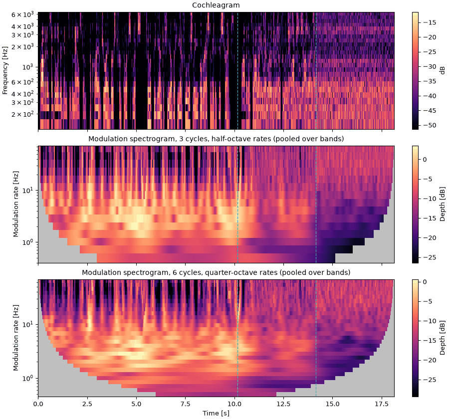
Three sentences from two talkers, then 4 s of babble made of six copies of the same sentences
overlapping at random, then 4 s of noise with the sentences' long-term spectrum. Speech is
modulated most strongly between about 2 and 8 Hz, the rate of its syllables (Greenberg & Kingsbury,
1997). That rhythm is what babble partly hides and
speech-shaped noise lacks entirely.
Code
names = ("bdl_arctic_a0131", "rms_arctic_a0132", "rms_arctic_a0133")
sentences = [so.load(f"docs/speech/{n}.flac").normalize(rms=0.1) for n in names]
talk = so.concat(sentences)
n = int(4 * fs)
babble = np.zeros(n)
for s in sentences * 2:
    x = np.tile(s.data[:, 0], 3)
    start = int(rng.uniform(0, 1.5) * fs)
    babble[start:] += x[: n - start]
ssn = so.long_term_spectrum(sentences).to_sound(4, fs, rng=0)
mixed = so.concat([talk, so.Sound(babble, fs).normalize(rms=0.1), ssn.normalize(rms=0.1)])
marks = [talk.duration, talk.duration + 4]
print(f"sentences {talk.duration:.2f} s, then babble and noise, {mixed.duration:.2f} s in all")
sentences 10.14 s, then babble and noise, 18.14 s in all
Speech, babble and noise
The dashed lines mark where the babble and the noise begin. Under the sentences the pooled
depth is high from about 2 to 10 Hz, brightest around 3 to 5 Hz. In the babble it is weaker and
patchier, since six talkers' syllables fill each other's gaps. In the speech-shaped noise it
falls to the level any noise has: the envelope of a narrow band of noise fluctuates randomly,
more at rates near the band's width. Watch the image beside the player change at each line.
s1_speech_babble_and_noise.flac, 18.1 s, mono
Code
sound = finish(mixed)
fig, playhead, live = show(sound, marks=marks, start=1.5)
A higher voice
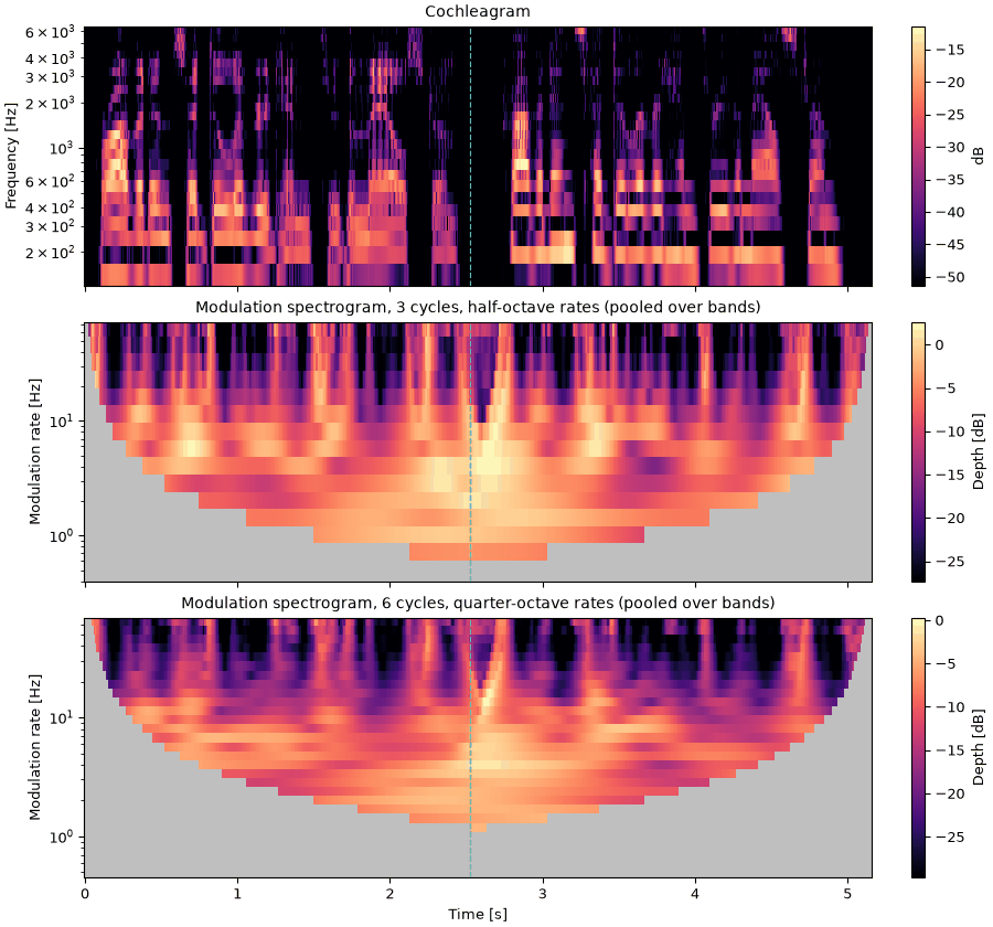
The first of those sentences read twice, by the male talker from the sentences above (bdl) and by
a female talker (slt) whose voice is roughly an octave higher. A spectrogram of the two looks
quite different, with the female talker's harmonics twice as far apart. Their modulation
spectrograms should not, if the modulation is set by the syllables rather than by the voice.
Code
same_sentence = [so.load(f"docs/speech/{n}_arctic_a0131.flac").normalize(rms=0.1) for n in ("bdl", "slt")]
two_voices = so.concat(same_sentence)
env, msg, fine = analyze(two_voices)
depth_db = 20 * np.log10(msg.depth[0])
depth_db[~msg.valid] = np.nan
switch = same_sentence[0].duration
for speaker, during in (("bdl", msg.t < switch), ("slt", msg.t >= switch)):
    pooled = np.nanmedian(depth_db[:, :, during], axis=(0, 2))
    rates = (msg.fm >= 2) & (msg.fm <= 16)
    pairs = zip(msg.fm[rates], pooled[rates], strict=True)
    shown = ", ".join(f"{rate:.3g} Hz {level:.1f}" for rate, level in pairs)
    print(f"{speaker}, median depth [dB]: {shown}")
The dashed line marks where the female talker begins; the bright patch around it is the pause
between the two readings, which every window that spans it reads as deep modulation. Away from the
line the pooled depth has the same shape in both halves, highest between about 2 and 8 Hz and
falling off above 10 Hz. The printout above gives the medians, which differ by 2 dB or less; the
male talker's are a little deeper at the slowest rates. Pitch does not show at all: the fastest
rate here, 64 Hz, is below either voice's F0, so the beating of harmonics within a band, at the
rate of F0, falls off the top. What does change is the cochleagram, whose low bands resolve the
female talker's widely spaced harmonics into separate stripes.
sound = finish(two_voices)
fig, playhead, live = show(sound, marks=[switch], start=1.2)
Three textures
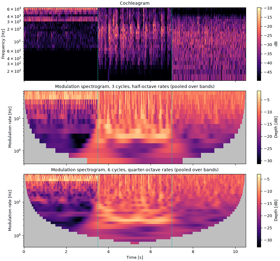
Crickets, applause and rain, 3.5 s of each, from the recordings on the
Sound textures page. A texture is a sound whose statistics stay put, so its
modulation spectrogram should hold still while each texture lasts and change at the joins.
Code
textures = [so.load(f"docs/textures/{n}.flac").resample(fs) for n in ("crickets", "applause", "rain")]
three = so.concat([s[:3.5].normalize(rms=0.1) for s in textures])
Crickets, applause and rain
The crickets chirp in pulses at about 40 to 60 Hz, and their modulation sits there and
nowhere else. Applause is a crowd of claps, each clapper about four times a second, and adds a
band of slow modulation. Rain has many small drops at no particular rate and the weakest
modulation of the three. The 6-cycle view separates the rates more cleanly, since nothing here
changes quickly.
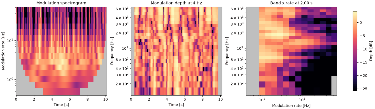
msg.slices(t, rate) draws three cuts through the cube at once, on one colour scale: rate
against time pooled over bands, frequency against time at one rate, and frequency against
rate at one moment. Here they are for the sentences, at 4 Hz and at 2 s.
Three cuts through the sentences
The middle panel shows which bands carry the 4 Hz rhythm and when: nearly all of them, in
step with the syllables, since a syllable's onset raises the level across the spectrum. On the
right, the moment at 2 s: depth is high from 1 to about 5 Hz in most bands and falls off above
10 Hz, most steeply in the low bands. The grey column is 0.5 Hz, whose 6 s window runs past
the start; the grey cell at the bottom right is 64 Hz in the lowest band, faster than that band
is wide.
Code
env, msg, fine = analyze(finish(talk))
fig = msg.slices(2.0, rate=4.0)
What this page leaves out
Power. Each cell also has a modulation power, |2y|^2, which says how much of the sound a modulation is rather than how modulated a band is (msg.power, and msg.average() over time). Pooled over bands it is dominated by the loudest bands and reads less clearly than depth.
Live analysis. With align="causal" every window ends at the time it reports, as a live analysis would see the sound, at the cost of a delay of half a window. The analysis can run on blocks of a stream and give the same numbers; a streaming version is planned.
Inversion. The phase of each filter output is dropped and the local mean divided out, so the modulation spectrogram can't be turned back into sound. To change a sound's modulation, filter its envelopes and resynthesize, as on the Analysis and resynthesis page.
The front end. Any filterbank's envelopes will do. A gammatone bank gives nearly the same pictures as the ERB bank used here; compressing the envelopes (raising them to the 0.3 power, as a cochlea does) scales every depth by about the same factor, 0.45.
Dau, Kollmeier & Kohlrausch (1997). Modeling auditory processing of amplitude modulation. I. Detection and masking with narrow-band carriers. JASA 102(5), 2892–2905. PubMed. Modulation filters a few cycles long. modulation.HannModulationFilterbank
Kingsbury, Morgan & Greenberg (1998). Robust speech recognition using the modulation spectrogram. Speech Communication 25(1–3), 117–132. doi:10.1016/S0167-6393(98)00032-6.
Kominek & Black (2004). The CMU Arctic speech databases. Proc. 5th ISCA Speech Synthesis Workshop, 223–224. ISCA Archive. The sentences, by speakers bdl, rms and slt.