Cepstral analysis

The sentence, and code the examples share

Every cepstrum below is taken from an STFT with Hann windows 40 ms long, every 5 ms. A window must hold about three periods for the harmonics to show as a ripple, and 40 ms is three periods at 75 Hz, below this speaker's lowest pitch.

import matplotlib.pyplot as plt
import numpy as np
from scipy.fft import dct, idct

import sonore as so
from sonore.core.utils import freq_to_mel
from sonore.views.mfcc import mel_filterbank

plt.rcParams.update({"font.size": 9, "axes.titlesize": 10, "figure.dpi": 100})


def finish(snd):
    """How every sound in the gallery is played: 5 ms ramps, RMS 0.1, peak at most 0.95."""
    snd = snd.ramp(5e-3).normalize(rms=0.1)
    return snd.normalize(peak=0.95) if snd.peak > 0.95 else snd


# The sentence at its native 16 kHz, and its F0 track (WORLD Harvest, 0 where unvoiced).
# Sources: docs/speech/SOURCES.md.
sentence = finish(so.load("docs/speech/bdl_arctic_a0131.flac"))
f0_times, f0_harvest = np.loadtxt("docs/speech/bdl_arctic_a0131_f0.csv", delimiter=",", skiprows=2).T
fs = sentence.fs

stft = so.STFT(sentence, win_dur=0.040, hop_dur=0.005)
cep = so.Cepstrum(stft)
FMAX = 5000

One time window

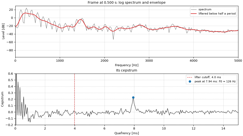
Take one time window in the middle of a vowel. Its log spectrum is a comb of harmonics riding on the formant envelope. Its cepstrum has most of its weight in the first couple of milliseconds, and one clear peak at the pitch period. Keeping only the quefrencies below half a period (a lifter, the cepstral counterpart of a filter) and transforming back gives the smooth envelope.

One time window

Top: the time window's log spectrum and the liftered envelope. Bottom: its cepstrum, with the peak at one period. The envelope runs a few dB under the harmonic peaks because the lifter averages the peaks with the dips between them; spectral-envelope estimators such as WORLD's CheapTrick correct for this (Morise, 2015).

Code

i = int(np.argmin(np.abs(cep.t - 0.50)))
_, f0_all, peak_all = cep.f0()
t_window, f0_window, peak_window = cep.t[i], f0_all[0, i], peak_all[0, i]
cutoff = 0.5 / f0_window  # half a period
envelope = cep.lifter(cutoff).envelope()[0, :, i]

fig, (ax0, ax1) = plt.subplots(2, 1, figsize=(10, 5.6), layout="constrained")
ax0.plot(stft.f, 20 * np.log10(np.abs(stft.data[0, :, i])), color="0.4", lw=0.8, label="spectrum")
ax0.plot(stft.f, 20 * np.log10(envelope), color="tab:red", lw=1.6, label="liftered below half a period")
ax0.set(
    xlim=(0, FMAX),
    xlabel="Frequency [Hz]",
    ylabel="Level [dB]",
    title=f"Time window at {t_window:.3f} s: log spectrum and envelope",
)
ax0.legend(loc="upper right", fontsize=8)
q_ms = cep.q * 1e3
ax1.plot(q_ms, cep.data[0, :, i], color="k", lw=0.8)
ax1.axvline(cutoff * 1e3, color="tab:red", ls="--", lw=1, label=f"lifter cutoff, {cutoff * 1e3:.1f} ms")
peak_label = f"peak at {1e3 / f0_window:.2f} ms: F0 = {f0_window:.0f} Hz"
ax1.plot(1e3 / f0_window, peak_window, "o", color="tab:blue", label=peak_label)
ax1.set(xlim=(0, 15), ylim=(-0.2, 0.6), xlabel="Quefrency [ms]", ylabel="Cepstrum", title="Its cepstrum")
ax1.legend(loc="upper right", fontsize=8)
for ax in (ax0, ax1):
    ax.grid(ls=":")

Pitch from the cepstrum

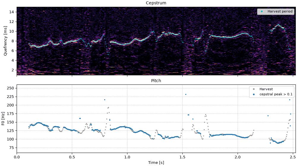
Doing this for every time window gives a cepstrogram: time across, quefrency up. Wherever the voice is voiced, a bright line runs at one period, falling as the pitch rises. Picking the largest peak between 2.5 and 13.3 ms (400 and 75 Hz) in each time window is classic cepstral pitch estimation (Noll, 1967). A time window counts as voiced when its peak is taller than 0.1.

The cepstrogram and its pitch

Top: the cepstrogram, with Harvest's pitch period drawn over it. Bottom: the cepstral F0 next to Harvest's. Each time window is judged on its own, with no continuity from one to the next, so the occasional time window jumps an octave.

c2_the_cepstrogram_and_its_pitch.flac, 2.5 s, mono

Code

t, f0_cep, peak = cep.f0(f_lo=75, f_hi=400)
voiced = f0_harvest > 0
fig, (ax0, ax1) = plt.subplots(2, 1, figsize=(10, 5.6), sharex=True, layout="constrained")
cep.plot(ax0, colorbar=False)
ax0.set_xlabel("")
ax0.plot(f0_times[voiced], 1e3 / f0_harvest[voiced], ".", ms=1.5, color="c", label="Harvest period")
ax0.legend(loc="upper right", fontsize=8, markerscale=4)
ax1.plot(f0_times[voiced], f0_harvest[voiced], ".", ms=3, color="0.6", label="Harvest")
ax1.plot(t[f0_cep[0] > 0], f0_cep[0][f0_cep[0] > 0], ".", ms=3, color="tab:blue", label="cepstral peak > 0.1")
ax1.set(ylim=(60, 260), xlabel="Time [s]", ylabel="F0 [Hz]", title="Pitch")
ax1.legend(loc="upper right", fontsize=8, markerscale=2)
ax1.grid(ls=":")
for ax in (ax0, ax1):
    ax.set_xlim(0, sentence.duration)
playhead = [ax0, ax1]
sound = sentence

harvest_at = np.interp(t, f0_times, f0_harvest)
both = (harvest_at > 0) & (f0_cep[0] > 0)
agree = np.mean(np.abs(f0_cep[0][both] / harvest_at[both] - 1) < 0.05)
print(f"time windows both call voiced: {both.sum()}; cepstral F0 within 5% of Harvest on {agree:.0%}")

time windows both call voiced: 318; cepstral F0 within 5% of Harvest on 96%

A tracker beside the cepstrum

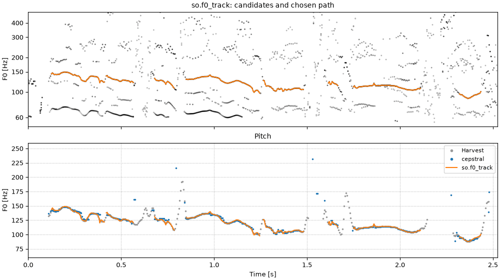
so.f0_track works the other way round. It looks for the period in the waveform rather than the log spectrum, with YIN's difference function (de Cheveigné & Kawahara, 2002): up to eight candidate periods per time window, each sharpened from the instantaneous frequencies of the first six harmonics, as WORLD does. Each candidate is scored by how well the waveform repeats one period later, and a single pass picks the cheapest path through the candidates, so that the pitch rarely jumps and a time window is voiced only when some candidate repeats well (a score above 0.5).

Cepstral F0, a tracker, and Harvest

Top: the tracker's candidates in grey, darker for a higher score, and the path it chose. The darkest row, an octave below the path, is the subharmonic: anything that repeats every period also repeats every two, so it scores as well, and the tracker never chooses a candidate when another at a whole multiple of its frequency scores about as well (subharmonic_margin). Bottom: the three pitch tracks together. Where the tracker and Harvest both call a time window voiced they agree; Harvest voices more time windows, stretches where the tracker's best score falls below 0.5. Against laryngograph recordings Harvest calls about a third of the unvoiced time windows voiced, which is why the tracker is stricter by default (see docs/design/views/f0.md).

f1_cepstral_f0_a_tracker_and_harvest.flac, 2.5 s, mono

Code

track = so.f0_track(sentence)
fig, (ax0, ax1) = plt.subplots(2, 1, figsize=(10, 5.6), sharex=True, layout="constrained")
track.plot(ax0, candidates=True, color="tab:orange")
ax0.set(ylim=(50, 500), yscale="log", xlabel="", title="so.f0_track: candidates and chosen path")
ax0.set_yticks([60, 100, 150, 200, 300, 400], labels=["60", "100", "150", "200", "300", "400"])
ax0.minorticks_off()
ax1.plot(f0_times[voiced], f0_harvest[voiced], ".", ms=3, color="0.6", label="Harvest")
ax1.plot(t[f0_cep[0] > 0], f0_cep[0][f0_cep[0] > 0], ".", ms=3, color="tab:blue", label="cepstral")
tracked = np.where(track.voiced[0], track.f0[0], np.nan)
ax1.plot(track.t, tracked, color="tab:orange", lw=1.5, label="so.f0_track")
ax1.set(ylim=(60, 260), xlabel="Time [s]", ylabel="F0 [Hz]", title="Pitch")
ax1.legend(loc="upper right", fontsize=8, markerscale=2)
ax1.grid(ls=":")
for ax in (ax0, ax1):
    ax.set_xlim(0, sentence.duration)
playhead = [ax0, ax1]
sound = sentence

# Compare at every time window of the tracker; the cepstrogram's time windows include them.
at = np.searchsorted(np.round(t, 6), np.round(track.t, 6))
pitch = {
    "Harvest": np.interp(track.t, f0_times, f0_harvest),
    "cepstral": f0_cep[0][at],
    "so.f0_track": np.where(track.voiced[0], track.f0[0], 0.0),
}
for name, f in pitch.items():
    print(f"{name:12s} voiced on {np.mean(f > 0):.0%} of time windows")
for a, b in [("cepstral", "Harvest"), ("so.f0_track", "Harvest"), ("cepstral", "so.f0_track")]:
    both = (pitch[a] > 0) & (pitch[b] > 0)
    agree = np.mean(np.abs(pitch[a][both] / pitch[b][both] - 1) < 0.05)
    print(f"{a} and {b}: both voiced on {both.sum()} time windows, within 5% on {agree:.0%}")

Harvest      voiced on 86% of time windows
cepstral     voiced on 65% of time windows
so.f0_track  voiced on 68% of time windows
cepstral and Harvest: both voiced on 318 time windows, within 5% on 96%
so.f0_track and Harvest: both voiced on 343 time windows, within 5% on 100%
cepstral and so.f0_track: both voiced on 300 time windows, within 5% on 98%

Splitting the voice in two

Lifter the other way and the two parts can be heard separately. Each time window keeps its own lifter cutoff, half of its pitch period, following Harvest's track (bridged across unvoiced stretches). Low quefrencies keep the vocal tract; high quefrencies keep the source.

voiced_t, voiced_f0 = f0_times[voiced], f0_harvest[voiced]
cutoffs = 0.5 / np.exp(np.interp(cep.t, voiced_t, np.log(voiced_f0)))  # half a period, per time window
tract = cep.lifter(cutoffs)  # low quefrencies: the envelope
source = cep.lifter(cutoffs, keep="high")  # high quefrencies: the harmonics
source.data[:, 0] = cep.data[:, 0]  # but keep each time window's mean log level, so pauses stay quiet


def show(snd, title, win_dur=0.005):
    fig, ax = plt.subplots(figsize=(10, 3.0), layout="constrained")
    so.STFT(snd, win_dur=win_dur, hop_dur=0.001).plot(ax, db_range=60, colorbar=False, fmax=FMAX)
    ax.set(xlim=(0, sentence.duration), title=f"{title} (Hann {win_dur * 1e3:g} ms spectrogram)")
    return fig, [ax]

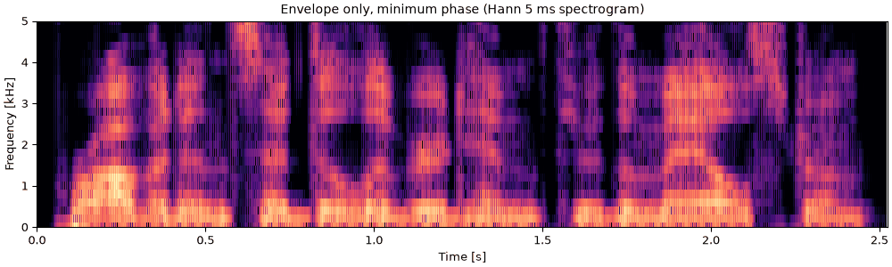
Envelope only, on a 200 Hz pulse train

The vocal tract alone: every time window's envelope given its minimum phase, so that each time window becomes one short pulse at its center. The time windows are 5 ms apart, so the pulses make a steady 200 Hz buzz. The words survive; the intonation does not.

c3_envelope_only_on_a_200_hz_pulse_train.flac, 2.5 s, mono

Code

robot = finish(tract.to_sound(phase="minimum"))
fig, playhead = show(robot, "Envelope only, minimum phase")
sound = robot

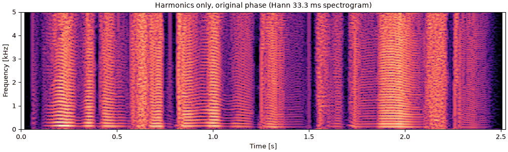
Harmonics only, the envelope flattened

The source alone: the high quefrencies, plus each time window's overall level, with the original phase. The formants are flattened away, leaving the harmonics at roughly equal level, a buzzy voice that still carries the talker's intonation. The narrowband spectrogram shows the harmonics running flat across frequency.

c4_harmonics_only_the_envelope_flattened.flac, 2.5 s, mono

Code

flat = finish(source.to_sound(phase="original"))
fig, playhead = show(flat, "Harmonics only, original phase", win_dur=0.0333)
sound = flat

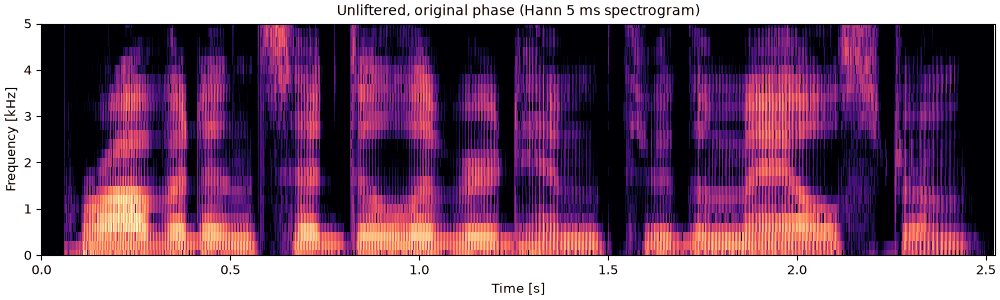
Both parts together

For comparison, both parts put back together: an unliftered cepstrum resynthesizes the sentence to rounding error.

c5_both_parts_together.flac, 2.5 s, mono

Code

whole = cep.to_sound()
print(f"largest difference from the sentence: {np.abs(whole.data - sentence.data).max():.1e}")
fig, playhead = show(whole, "Unliftered, original phase")
sound = finish(whole)

A higher voice

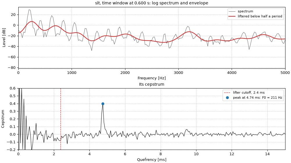
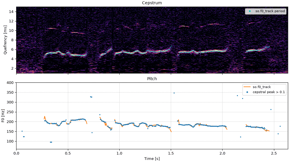
The same sentence read by a female talker (CMU ARCTIC, speaker slt), whose pitch sits around 180 to 210 Hz, half as high again as the male talker's. Two things change in the cepstrum. The pitch peak moves down to about 5 ms, closer to the envelope's first couple of milliseconds, though still clear of them. And a lifter at half a period now keeps only the quefrencies below about 2.5 ms, against 4 ms for the male talker, so the envelope it recovers is smoother and follows the formants less closely: with harmonics further apart, there is less of the envelope to recover. On a database of laryngograph recordings, cepstral F0 made octave-down errors on 1.5% of a female voice's time windows and none on a male voice's (docs/design/views/female-voices.md). There is no stored F0 track for this recording, so so.f0_track stands in for Harvest.

sentence_female = finish(so.load("docs/speech/slt_arctic_a0131.flac"))
stft_female = so.STFT(sentence_female, win_dur=0.040, hop_dur=0.005)
cep_female = so.Cepstrum(stft_female)
t_female, f0_cep_female, peak_female = cep_female.f0(f_lo=75, f_hi=400)
track_female = so.f0_track(sentence_female)

One time window, a higher voice

One time window of the female talker's sentence, drawn as for the male talker's above. The harmonics are further apart, so the log spectrum ripples less often, and the cepstral peak sits at a shorter quefrency. The lifter cutoff, at half the female period, is lower too.

Code

i_female = int(np.argmin(np.abs(t_female - 0.60)))
f0_window_female = f0_cep_female[0, i_female]
cutoff_female = 0.5 / f0_window_female
envelope_female = cep_female.lifter(cutoff_female).envelope()[0, :, i_female]

fig, (ax0, ax1) = plt.subplots(2, 1, figsize=(10, 5.6), layout="constrained")
spectrum_db = 20 * np.log10(np.abs(stft_female.data[0, :, i_female]))
ax0.plot(stft_female.f, spectrum_db, color="0.4", lw=0.8, label="spectrum")
ax0.plot(
    stft_female.f,
    20 * np.log10(envelope_female),
    color="tab:red",
    lw=1.6,
    label="liftered below half a period",
)
ax0.set(
    xlim=(0, FMAX),
    xlabel="Frequency [Hz]",
    ylabel="Level [dB]",
    title=f"slt, time window at {t_female[i_female]:.3f} s: log spectrum and envelope",
)
ax0.legend(loc="upper right", fontsize=8)
ax1.plot(cep_female.q * 1e3, cep_female.data[0, :, i_female], color="k", lw=0.8)
ax1.axvline(
    cutoff_female * 1e3, color="tab:red", ls="--", lw=1, label=f"lifter cutoff, {cutoff_female * 1e3:.1f} ms"
)
peak_label = f"peak at {1e3 / f0_window_female:.2f} ms: F0 = {f0_window_female:.0f} Hz"
ax1.plot(1e3 / f0_window_female, peak_female[0, i_female], "o", color="tab:blue", label=peak_label)
ax1.set(xlim=(0, 15), ylim=(-0.2, 0.6), xlabel="Quefrency [ms]", ylabel="Cepstrum", title="Its cepstrum")
ax1.legend(loc="upper right", fontsize=8)
for ax in (ax0, ax1):
    ax.grid(ls=":")

The cepstrogram of a higher voice

Top: the female talker's cepstrogram, with the tracker's pitch period drawn over it; the bright line runs lower than the male talker's. Bottom: cepstral F0 beside so.f0_track.

c7_the_cepstrogram_of_a_higher_voice.flac, 2.6 s, mono

Code

voiced_female = track_female.voiced[0]
fig, (ax0, ax1) = plt.subplots(2, 1, figsize=(10, 5.6), sharex=True, layout="constrained")
cep_female.plot(ax0, colorbar=False)
ax0.set_xlabel("")
period_ms = 1e3 / track_female.f0[0][voiced_female]
ax0.plot(track_female.t[voiced_female], period_ms, ".", ms=1.5, color="c", label="so.f0_track period")
ax0.legend(loc="upper right", fontsize=8, markerscale=4)
tracked_female = np.where(voiced_female, track_female.f0[0], np.nan)
cep_voiced = f0_cep_female[0] > 0
ax1.plot(track_female.t, tracked_female, color="tab:orange", lw=1.5, label="so.f0_track")
ax1.plot(
    t_female[cep_voiced],
    f0_cep_female[0][cep_voiced],
    ".",
    ms=3,
    color="tab:blue",
    label="cepstral peak > 0.1",
)
ax1.set(ylim=(60, 400), xlabel="Time [s]", ylabel="F0 [Hz]", title="Pitch")
ax1.legend(loc="upper right", fontsize=8, markerscale=2)
ax1.grid(ls=":")
for ax in (ax0, ax1):
    ax.set_xlim(0, sentence_female.duration)
playhead = [ax0, ax1]
sound = sentence_female

at_female = np.searchsorted(np.round(t_female, 6), np.round(track_female.t, 6))
cep_at_track = f0_cep_female[0][np.minimum(at_female, len(t_female) - 1)]
tracked_hz = np.where(voiced_female, track_female.f0[0], 0.0)
both = (cep_at_track > 0) & (tracked_hz > 0)
ratio = cep_at_track[both] / tracked_hz[both]
print(f"median F0 (so.f0_track): {np.median(tracked_hz[tracked_hz > 0]):.0f} Hz")
agree_female = np.mean(np.abs(ratio - 1) < 0.05)
print(
    f"both voiced on {both.sum()} time windows; cepstral F0 within 5% of the tracker on {agree_female:.0%},"
)
print(f"an octave below on {np.mean(np.abs(ratio - 0.5) < 0.05):.1%}")

median F0 (so.f0_track): 183 Hz
both voiced on 333 time windows; cepstral F0 within 5% of the tracker on 96%,
an octave below on 0.9%

MFCCs: a cepstrum on the mel scale

Speech recognisers have long described each time window by its mel-frequency cepstral coefficients (Davis & Mermelstein, 1980). The recipe is the cepstrum's, with one step put in front: the power spectrum is first summed into a few dozen triangular bands spaced evenly on the mel scale, a frequency scale that is roughly linear below 1 kHz and logarithmic above, as the ear's resolution is. Then the logarithm, and a cosine transform (a DCT) of the 26 log band powers in place of the Fourier transform. Keeping the first 13 coefficients is a lifter, as in One time window: it keeps the slow shape across the bands and drops the fine detail. so.MFCC follows the HTK and Kaldi speech recipe by default: 25 ms Hamming windows every 10 ms, 26 bands up to half the sampling rate, 13 coefficients.

The aim is to keep the vocal tract and drop the pitch. The bands and the lifter both smooth over the harmonics, but not completely: the lowest bands are narrower than the gap between harmonics of a higher voice, so some sit on a harmonic and their neighbours between two, and the pitch leaks back into the coefficients. A vowel synthesised with a known vocal tract shows how much.

# Two vowels as sums of harmonics, each harmonic weighted by a vocal tract of four resonances
# (rounded Peterson & Barney, 1952, male averages; bandwidths chosen here), so the true
# envelope is known exactly.
FORMANTS = {
    "a": [(730, 60), (1090, 100), (2440, 120), (3400, 175)],
    "i": [(270, 60), (2290, 100), (3010, 120), (3400, 175)],
}


def tract_gain(freqs, vowel):
    """The vocal tract's |H(f)|: a cascade of second-order resonators."""
    z = np.exp(-2j * np.pi * np.asarray(freqs, dtype=float) / fs)
    denominator = np.ones_like(z)
    for centre, bandwidth in FORMANTS[vowel]:
        radius = np.exp(-np.pi * bandwidth / fs)
        denominator *= 1 - 2 * radius * np.cos(2 * np.pi * centre / fs) * z + radius**2 * z**2
    return 1 / np.abs(denominator)


def synthetic_vowel(f0, vowel, duration=0.4):
    times = np.arange(round(duration * fs)) / fs
    harmonic_freqs = f0 * np.arange(1, int(0.45 * fs / f0) + 1)
    amplitudes = tract_gain(harmonic_freqs, vowel)
    waves = amplitudes[:, None] * np.cos(2 * np.pi * harmonic_freqs[:, None] * times)
    return so.Sound(waves.sum(0), fs)


def keep_13(band_power):
    """Band powers to 13 MFCCs and back: the log band powers the coefficients keep."""
    coefficients = dct(np.log(band_power), type=2, norm="ortho", axis=0)
    coefficients[13:] = 0
    return idct(coefficients, type=2, norm="ortho", axis=0)


f_plot = np.linspace(0, FMAX, 1001)
f0s = (100, 150, 200, 250, 300)
smoothed = {}  # (source, vowel, F0): the 13-coefficient log band powers, level removed
for vowel in FORMANTS:
    for f0 in f0s:
        vowel_sound = synthetic_vowel(f0, vowel)
        mfcc_vowel = so.MFCC(vowel_sound)
        middle = len(mfcc_vowel.t) // 2
        envelope_vowel = so.cheaptrick(
            vowel_sound, (mfcc_vowel.t[middle : middle + 1], np.array([float(f0)]))
        )
        envelope_freqs = np.arange(envelope_vowel.n_fft // 2 + 1) * fs / envelope_vowel.n_fft
        envelope_weights, _ = mel_filterbank(26, envelope_freqs, 0, fs / 2)
        for source_name, band_power in (
            ("power spectrum", mfcc_vowel.mel_power[0, :, middle]),
            ("CheapTrick envelope", envelope_weights @ envelope_vowel.data[0, :, 0]),
        ):
            log_power = keep_13(band_power)
            smoothed[source_name, vowel, f0] = log_power - log_power.mean()
band_mels = freq_to_mel(mfcc_vowel.cfs)
true_db = 20 * np.log10(tract_gain(f_plot, "a"))


def on_plot_axis(log_power):
    """13-coefficient log band powers in dB, drawn between the band centres as so.MFCC.envelope
    does (linear in mel), and shifted to the true envelope's mean level from 100 Hz up."""
    level_db = 10 / np.log(10) * np.interp(freq_to_mel(f_plot), band_mels, log_power)
    above_100 = f_plot >= 100
    return level_db + np.mean(true_db[above_100] - level_db[above_100])

One vowel at three pitches

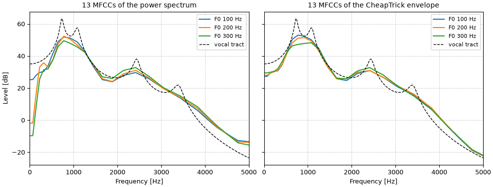
The vowel /a/ at three pitches, each analysed in one 25 ms time window. Left: the 13 MFCCs of its power spectrum, drawn back as an envelope (as mfcc.envelope(f) does). Right: the same 13 coefficients taken from CheapTrick's envelope instead, summed into the same mel bands. Dashed: the vocal tract the harmonics were weighted by. Levels are matched to it, since only the shape matters here (the level is c0). From the power spectrum, the lowest bands, below the first harmonic of the 200 and 300 Hz voices, drop by 30 dB and more, and the first formant changes shape with the pitch. CheapTrick has already smoothed over one harmonic spacing, so the three curves nearly coincide. The 13 coefficients cannot follow the formant peaks at any of the pitches: that is the lifter, and it is the same for all three.

Code

fig, axes = plt.subplots(1, 2, figsize=(10, 3.8), sharey=True, layout="constrained")
for ax, source_name in zip(axes, ("power spectrum", "CheapTrick envelope"), strict=True):
    for f0, color in zip((100, 200, 300), ("tab:blue", "tab:orange", "tab:green"), strict=True):
        ax.plot(
            f_plot, on_plot_axis(smoothed[source_name, "a", f0]), color=color, lw=1.5, label=f"F0 {f0} Hz"
        )
    ax.plot(f_plot, true_db, "k--", lw=1, label="vocal tract")
    ax.set(xlim=(0, FMAX), xlabel="Frequency [Hz]", title=f"13 MFCCs of the {source_name}")
    ax.legend(loc="upper right", fontsize=8)
    ax.grid(ls=":")
axes[0].set_ylabel("Level [dB]")

The distance between two such curves, the rms difference over the 26 bands in dB, puts a number on it. Between F0s of 100 to 300 Hz the same vowel moves about a third as far as the change from /a/ to /i/; taken from CheapTrick's envelope, about a tenth as far.

def distance_db(first, second):
    return 10 / np.log(10) * np.sqrt(np.mean((first - second) ** 2))


for source_name in ("power spectrum", "CheapTrick envelope"):
    same_vowel = [
        distance_db(smoothed[source_name, vowel, low], smoothed[source_name, vowel, high])
        for vowel in FORMANTS
        for low in f0s
        for high in f0s
        if low < high
    ]
    across = [distance_db(smoothed[source_name, "a", f0], smoothed[source_name, "i", f0]) for f0 in f0s]
    print(
        f"from the {source_name}: same vowel at two F0s, median {np.median(same_vowel):.1f} dB "
        f"(largest {max(same_vowel):.1f}); /a/ vs /i/ at one F0, {min(across):.1f} to {max(across):.1f} dB"
    )

from the power spectrum: same vowel at two F0s, median 5.6 dB (largest 9.2); /a/ vs /i/ at one F0, 15.4 to 17.6 dB
from the CheapTrick envelope: same vowel at two F0s, median 1.9 dB (largest 3.4); /a/ vs /i/ at one F0, 16.0 to 18.4 dB

The sentence as MFCCs

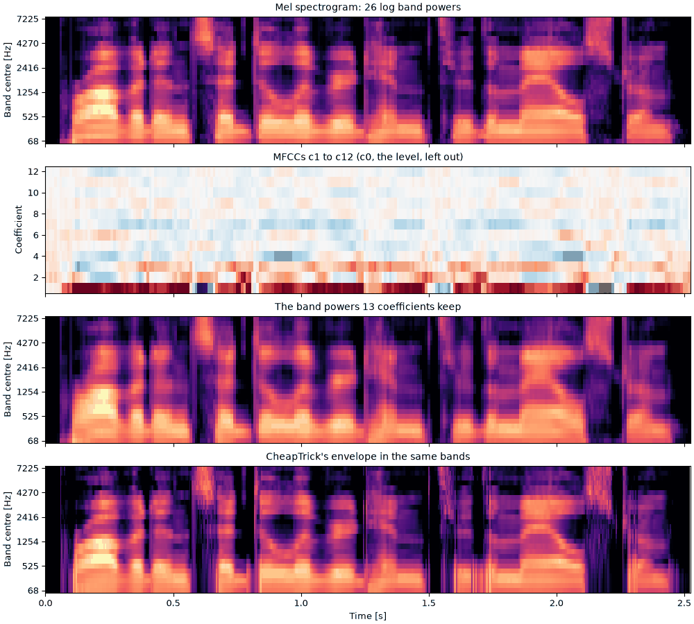
The sentence, analysed with so.MFCC(sentence). From the top: the 26 log band powers (the mel spectrogram, mfcc.plot(kind="mel")); the 13 coefficients, without c0, the level (mfcc.plot()); the band powers the 13 coefficients keep, drawn back from them; and CheapTrick's envelope on the same bands, from the so.f0_track pitch track above (unvoiced time windows are analysed as if at 500 Hz). The coefficients are hard to read by eye; drawn back, they are a mel spectrogram smoothed across the bands.

m2_the_sentence_as_mfccs.flac, 2.5 s, mono

Code

mfcc = so.MFCC(sentence)
envelope = so.cheaptrick(sentence, track)
envelope_freqs = np.arange(envelope.n_fft // 2 + 1) * fs / envelope.n_fft
envelope_weights, _ = mel_filterbank(26, envelope_freqs, 0, fs / 2)
band_rows = np.arange(len(mfcc.cfs))
row_ticks = band_rows[::5]


def band_image(ax, times, band_db, title):
    vmax = band_db.max()
    ax.pcolormesh(
        times, band_rows, band_db, cmap="magma", vmin=vmax - 60, vmax=vmax, shading="auto", rasterized=True
    )
    ax.set_yticks(row_ticks, [f"{mfcc.cfs[row]:.0f}" for row in row_ticks])
    ax.set(title=title, xlabel="", ylabel="Band centre [Hz]")


fig, axes = plt.subplots(4, 1, figsize=(10, 9), sharex=True, layout="constrained")
mfcc.plot(axes[0], kind="mel", colorbar=False)
axes[0].set(title="Mel spectrogram: 26 log band powers", xlabel="")
mfcc.plot(axes[1], colorbar=False)
axes[1].set(title="MFCCs c1 to c12 (c0, the level, left out)", xlabel="")
kept_db = 10 * np.log10(mfcc.envelope(mfcc.cfs)[0])
band_image(axes[2], mfcc.t, kept_db, "The band powers 13 coefficients keep")
band_image(
    axes[3],
    envelope.t,
    10 * np.log10(envelope_weights @ envelope.data[0]),
    "CheapTrick's envelope in the same bands",
)
axes[3].set_xlabel("Time [s]")
for ax in axes:
    ax.set_xlim(0, sentence.duration)
playhead = list(axes)
sound = sentence

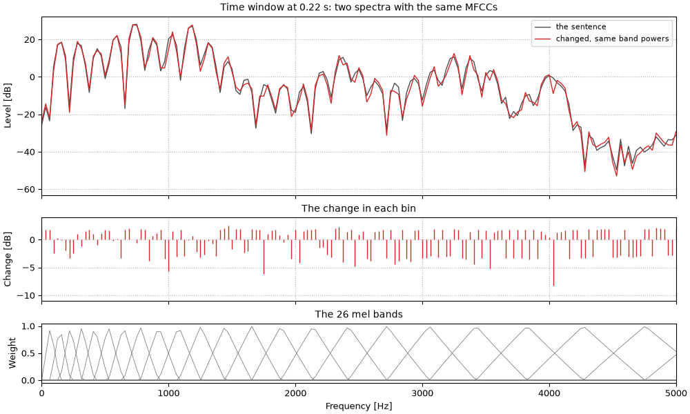
The mel bands and the cut to 13 coefficients both discard information, so MFCCs are a one-way view: no sound can be rebuilt from them, and many different spectra share the same coefficients. Within one band, power can move from one bin to another without the band's sum changing; with 257 bins and 26 bands there are 231 independent ways to do it.

Two spectra, one set of MFCCs

The loudest time window of the sentence, and the same spectrum with every bin's power changed by a factor between 0.1 and 1.9, in a direction that leaves all 26 band powers unchanged. Middle: the change in each bin. Bottom: the mel bands. The two spectra have the same MFCCs to rounding error.

Code

loudest = int(np.argmax(mfcc.mel_power[0].sum(0)))
power = np.abs(mfcc.source.data[0, :, loudest]) ** 2
# A relative change of each bin, at most 0.9, that no band sees: it lies in the null space of the
# band weights times the spectrum.
_, _, right_vectors = np.linalg.svd(mfcc.weights * power[None, :])
null_space = right_vectors[len(mfcc.cfs) :]
random_signs = np.random.default_rng(0).choice([-1.0, 1.0], power.size)
relative_change = null_space.T @ (null_space @ random_signs)
relative_change *= 0.9 / np.abs(relative_change).max()
gains = np.ones(mfcc.source.data.shape[1:])
gains[:, loudest] = np.sqrt(1 + relative_change)
mfcc_altered = so.MFCC(mfcc.source * gains)

bin_freqs = np.arange(mfcc.n_fft // 2 + 1) * fs / mfcc.n_fft
altered_power = np.abs(mfcc_altered.source.data[0, :, loudest]) ** 2
fig, (ax0, ax1, ax2) = plt.subplots(
    3, 1, figsize=(10, 6), sharex=True, height_ratios=[3, 1.4, 1], layout="constrained"
)
ax0.plot(bin_freqs, 10 * np.log10(power), color="0.3", lw=1, label="the sentence")
ax0.plot(bin_freqs, 10 * np.log10(altered_power), color="tab:red", lw=1, label="changed, same band powers")
ax0.set(ylabel="Level [dB]", title=f"Time window at {mfcc.t[loudest]:.2f} s: two spectra with the same MFCCs")
ax0.legend(loc="upper right", fontsize=8)
ax1.vlines(bin_freqs, 0, 10 * np.log10(altered_power / power), color="tab:red", lw=1)
ax1.set(ylim=(-11, 4), ylabel="Change [dB]", title="The change in each bin")
ax2.plot(bin_freqs, mfcc.weights.T, color="0.5", lw=0.6)
ax2.set(xlim=(0, FMAX), xlabel="Frequency [Hz]", ylabel="Weight", title="The 26 mel bands")
for ax in (ax0, ax1):
    ax.grid(ls=":")

change_db = np.abs(10 * np.log10(altered_power / power))
coefficient_change = np.abs(mfcc_altered.data[0, :, loudest] - mfcc.data[0, :, loudest]).max()
print(
    f"bins changed by more than 3 dB: {np.mean(change_db > 3):.0%}; "
    f"median change {np.median(change_db):.1f} dB"
)
print(f"largest change of any MFCC: {coefficient_change:.1e}")

bins changed by more than 3 dB: 30%; median change 1.9 dB
largest change of any MFCC: 8.9e-16

Reference implementations

so.Cepstrum is written from the definitions. tools/crosscheck_cepstrum.py compares it with three independent implementations; the numbers below are from SciPy 1.17.1 and Praat 6.1.38.

• **MATLAB rceps.** Its documented definition, real(ifft(log(abs(fft(x))))), written out in NumPy for one 40 ms time window, matches sonore's real cepstrum to 4e-16.
• **SciPy scipy.signal.minimum_phase** (method="homomorphic", half=False) builds a minimum-phase filter by the same folding of the real cepstrum. On a 17-tap mixed-phase filter it matches sonore's minimum phase to 4e-8 of the peak; SciPy adds a tiny constant to the magnitude before the log, which is the whole difference.
• Praat's PowerCepstrogram (Boersma & Weenink), through parselmouth, measures the same peak by a different route: a Gaussian window, the power spectrum in dB, and the sound resampled to 10 kHz. On the time windows of this sentence that sonore calls voiced, the two peaks agree within 5% on 98% of them; on every time window Harvest calls voiced, on 81%.

See also the design and its numerical checks, docs/design/views/cepstrum.md.

so.MFCC is tested against Kaldi's MFCCs (through kaldi-native-fbank, a re-implementation of Kaldi's feature code) to float32 precision, and against librosa's to 1e-8 of the largest coefficient; see docs/design/views/mfcc.md.

What this page leaves out

• Tracking from the cepstrum. Cepstral F0 judges each time window alone. The tracker above chooses a path through candidates from the waveform; the same could be done with cepstral peaks as the candidates.
• Better envelopes. A plain low lifter sits under the harmonic peaks; WORLD's CheapTrick smooths the spectrum over one F_0 first and corrects the lifter.
• Other cepstra on a warped axis. The mel-generalised cepstra of speech synthesis warp the frequency axis inside the cepstrum rather than with bands; PLP and gammatone cepstra use other auditory bands. MFCC deltas (mfcc.deltas()) are not shown.
• The complex cepstrum. It keeps the phase as well, but needs phase unwrapping, which is fragile on real sounds; sonore provides the real cepstrum and takes phase from the STFT or from the minimum-phase fold.

References

• Boersma & Weenink. Praat: doing phonetics by computer. praat.org.
• Bogert, Healy & Tukey (1963). The quefrency alanysis of time series for echoes: cepstrum, pseudo-autocovariance, cross-cepstrum and saphe cracking. In M. Rosenblatt (Ed.), Time Series Analysis. Wiley. Semantic Scholar. cepstrum.Cepstrum
• Davis & Mermelstein (1980). Comparison of parametric representations for monosyllabic word recognition in continuously spoken sentences. IEEE Trans. Acoust., Speech, Signal Process. 28(4), 357–366. mfcc.MFCC
• de Cheveigné & Kawahara (2002). YIN, a fundamental frequency estimator for speech and music. J. Acoust. Soc. Am. 111(4), 1917–1930. doi:10.1121/1.1458024. f0.f0_track
• Kominek & Black (2004). The CMU Arctic speech databases. Proc. 5th ISCA Speech Synthesis Workshop, 223–224. ISCA Archive. The sentence, by speakers bdl and slt.
• Morise (2015). CheapTrick, a spectral envelope estimator for high-quality speech synthesis. Speech Communication 67, 1–7. doi:10.1016/j.specom.2014.09.003. gabor.TVGaborFrame.pitch_adaptive
• Morise, Yokomori & Ozawa (2016). WORLD: a vocoder-based high-quality speech synthesis system for real-time applications. IEICE Trans. Inf. & Syst. E99-D(7), 1877–1884. doi:10.1587/transinf.2015EDP7457. Harvest.
• Peterson & Barney (1952). Control methods used in a study of the vowels. J. Acoust. Soc. Am. 24(2), 175–184. ASA. The formants of the synthetic vowels.
• Noll (1967). Cepstrum pitch determination. J. Acoust. Soc. Am. 41(2), 293–309. PubMed. cepstrum.Cepstrum.f0