Synthetic reverberation

import matplotlib.pyplot as plt
import numpy as np
from scipy.signal import butter, sosfilt

import sonore as so

plt.rcParams.update({"font.size": 9, "axes.titlesize": 10, "figure.dpi": 100})
FS = 44100


def finish(snd):
    """How every sound in the gallery is played: 5 ms ramps, RMS 0.1, peak at most 0.95."""
    snd = snd.ramp(5e-3).normalize(rms=0.1)
    return snd.normalize(peak=0.95) if snd.peak > 0.95 else snd


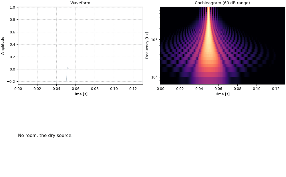
def starter_pistol():
    """A sharp broadband crack: a shock-like pulse (0.15 ms exponential), highpassed.
    Its spectrum is smooth; a short burst of noise would have random deep notches."""
    t = np.arange(int(0.03 * FS)) / FS
    x = sosfilt(butter(2, 300, "highpass", fs=FS, output="sos"), np.exp(-t / 0.15e-3))
    return so.Sound(x, FS).pad(before=0.05, after=0.05)


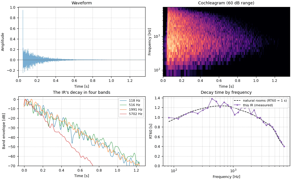
def room(**kw):
    """A synthetic room: RT60 1 s, direct-to-reverberant ratio -3 dB, a fixed seed."""
    return so.synth_ir(1.0, FS, drr_db=-3, rng=5, **kw)


def show(snd, ir, kw=None):
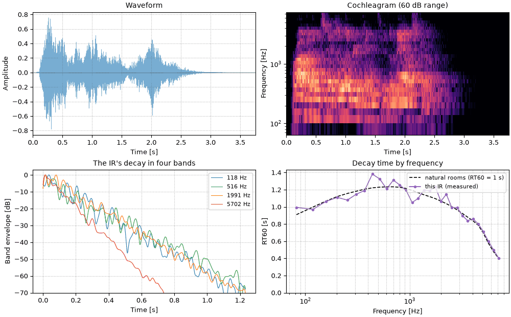
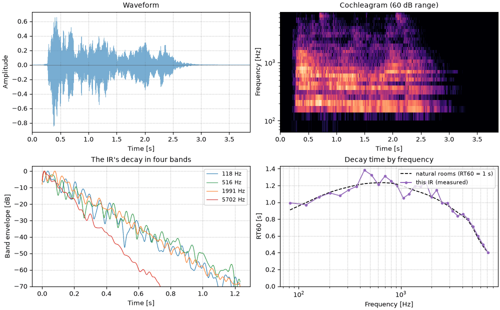
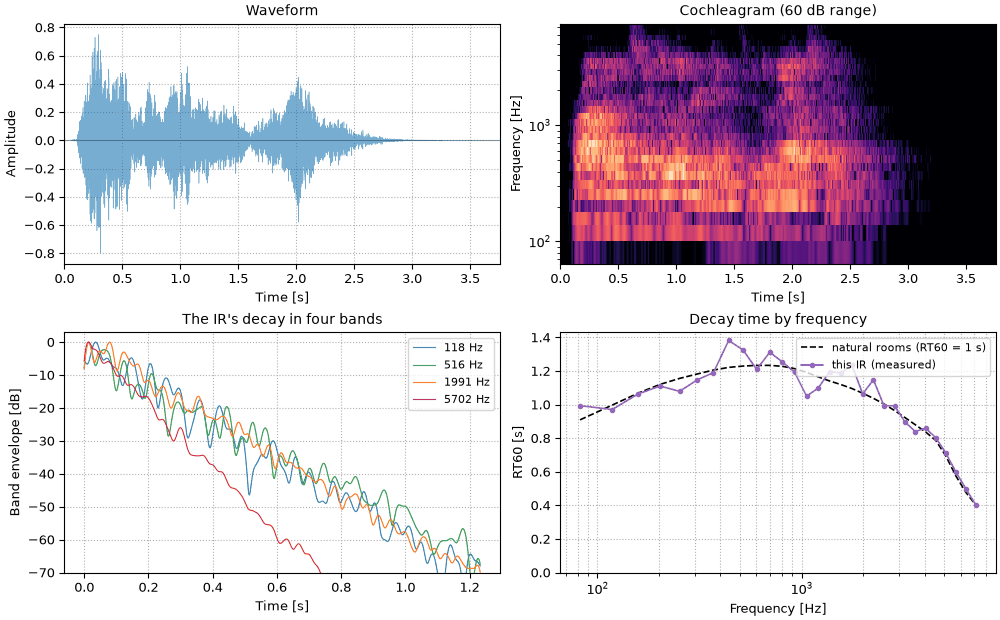
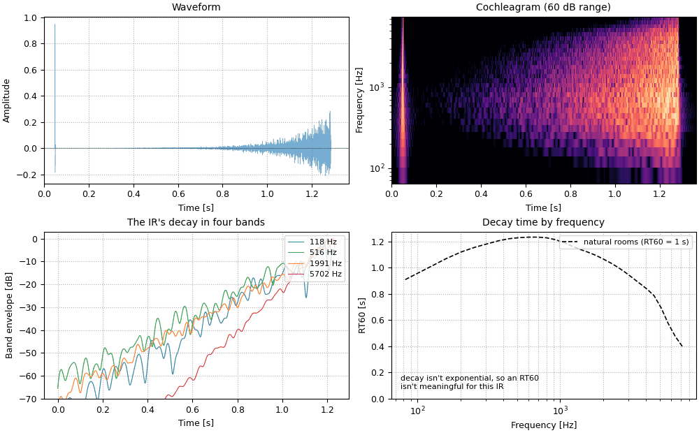
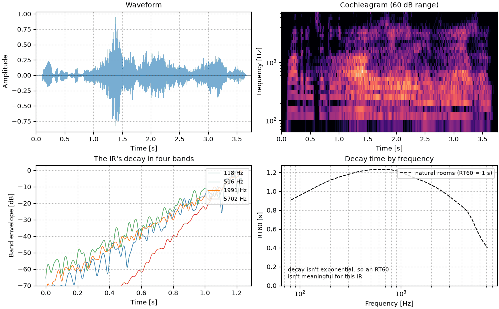
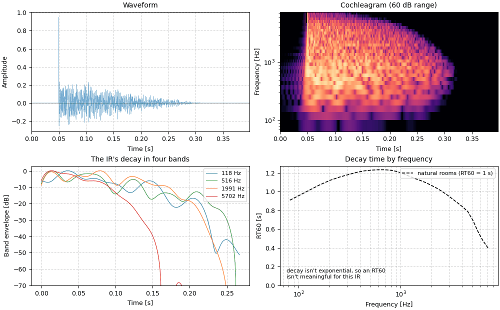
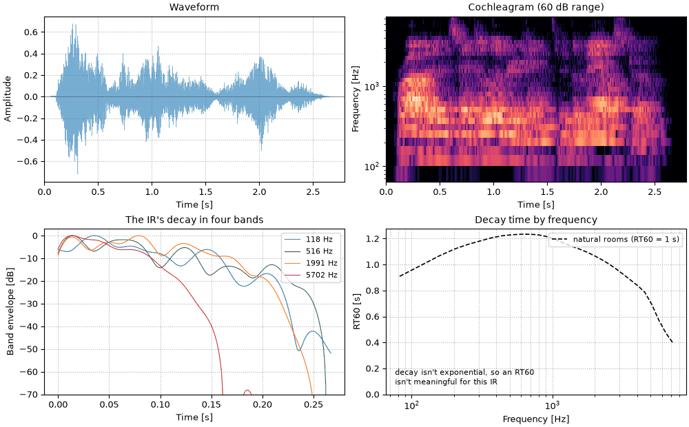
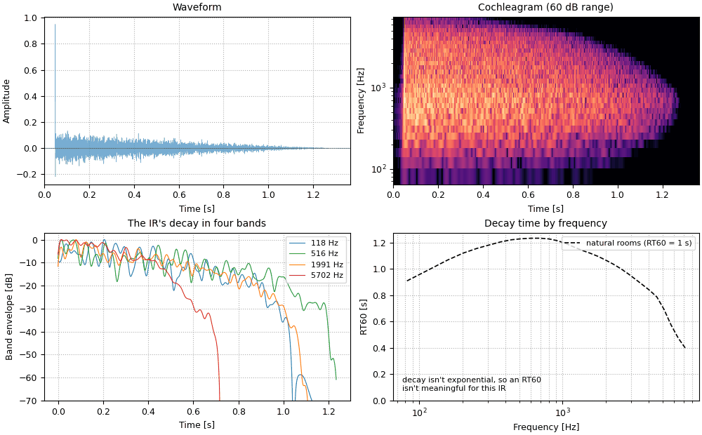
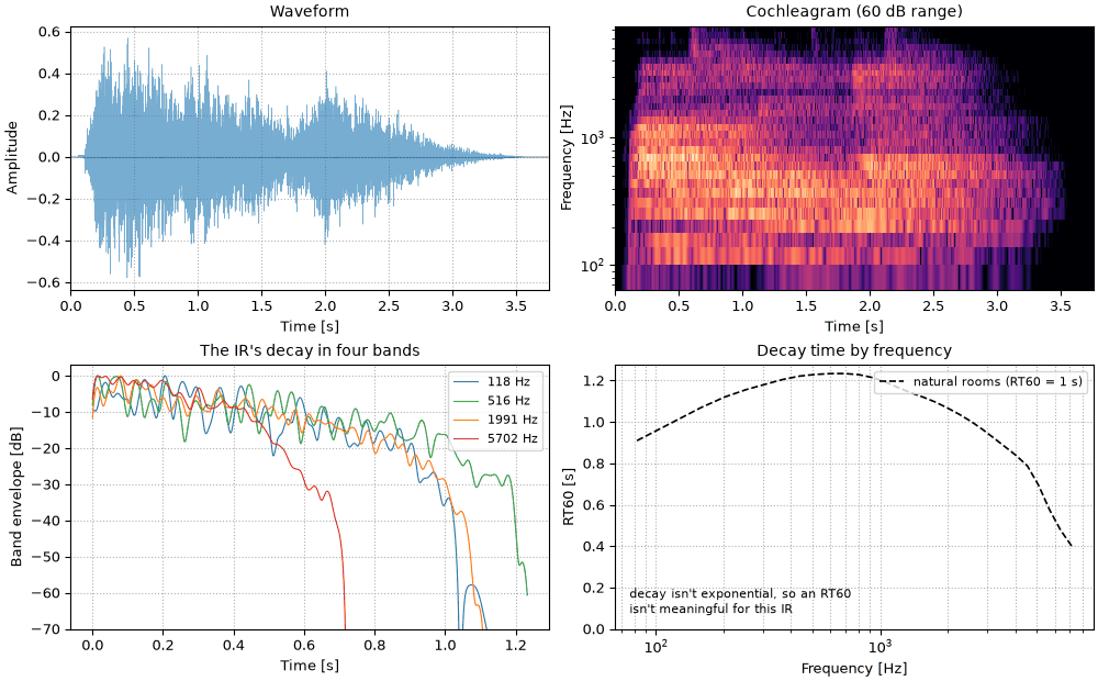
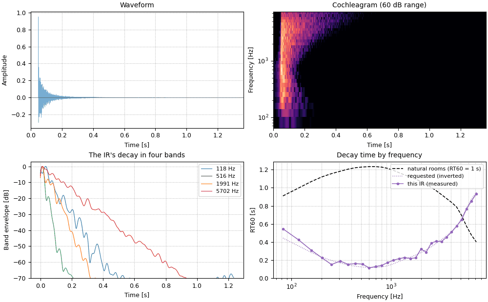
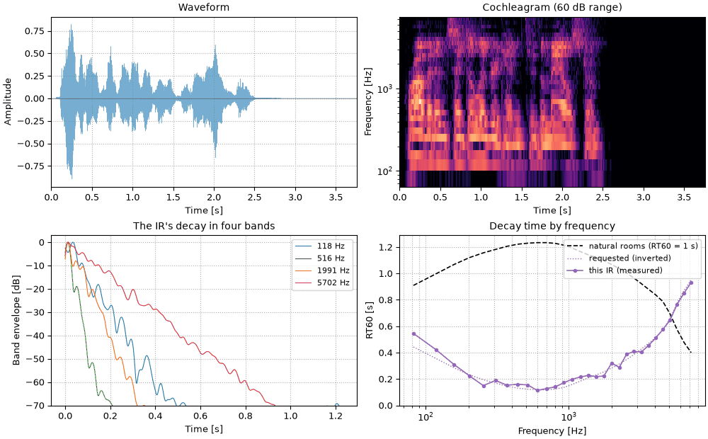
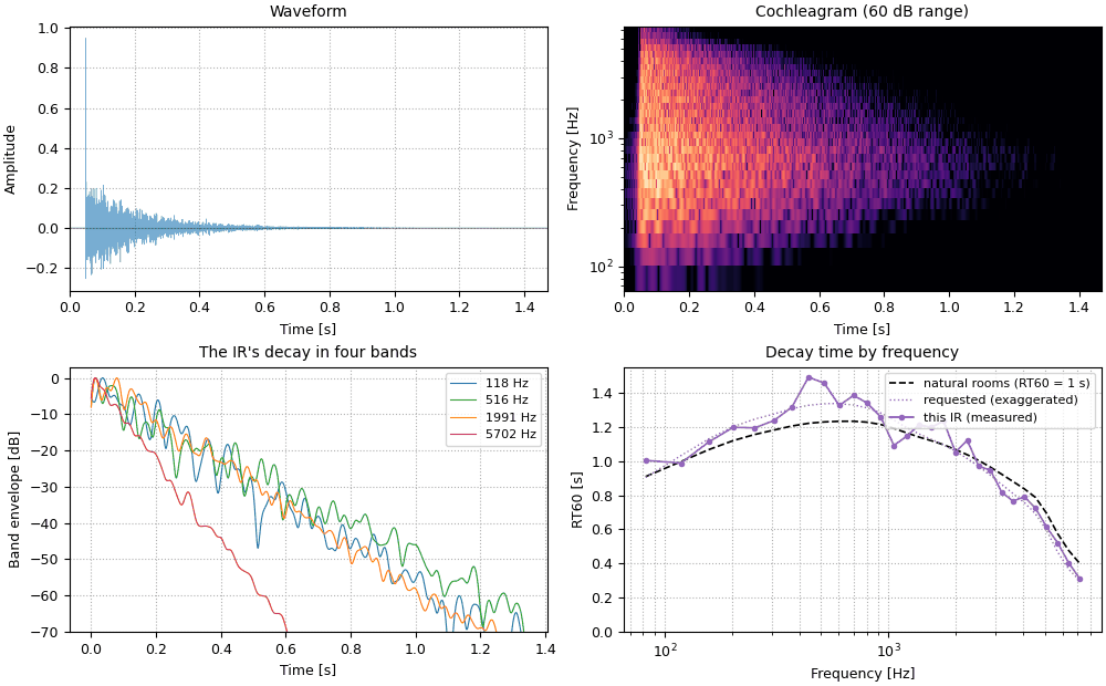
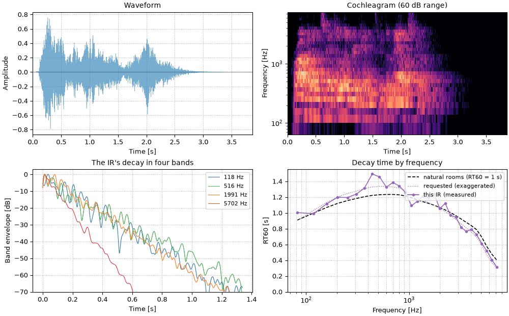
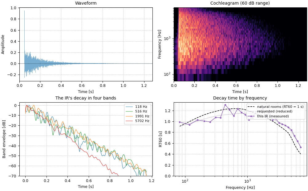
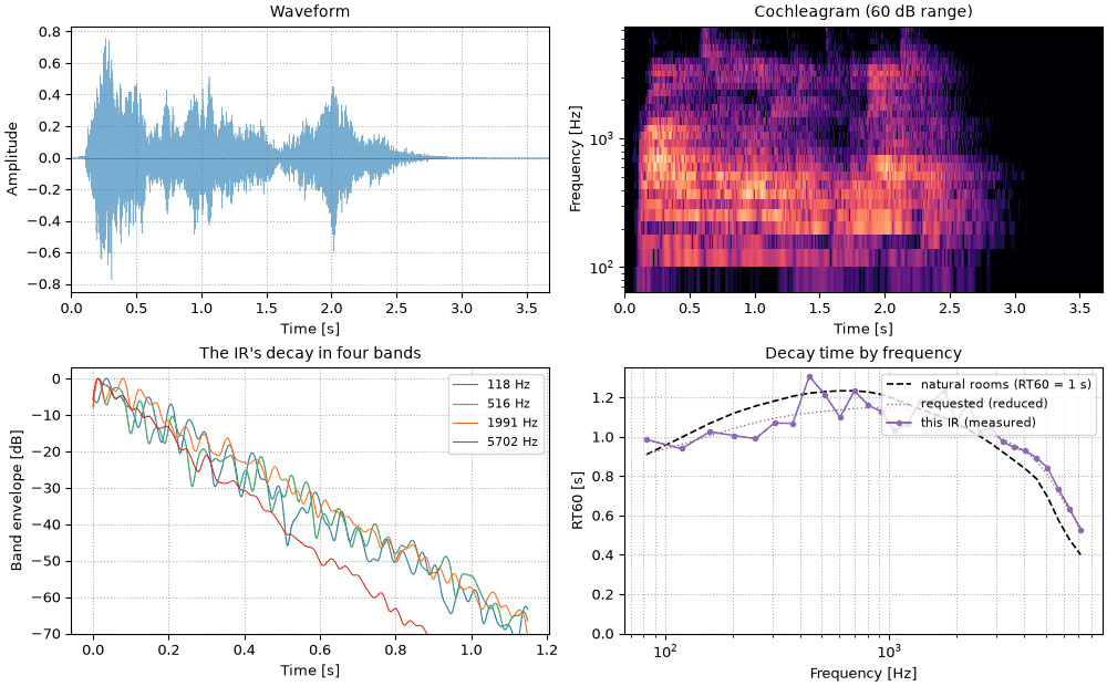
    """Waveform and cochleagram of the sound, then the IR's decay by band and its RT60s.
    Returns the figure and the panels the playhead follows."""
    fig, axes = plt.subplots(2, 2, figsize=(10, 6.2), layout="constrained")
    snd.plot(axes[0, 0], lw=0.4)
    axes[0, 0].set_title("Waveform")
    # no extra lowpass: resampling to 1 kHz is already band-limited, and a
    # lowpass would ring visibly around the sharp onset of the shot
    cochleagram = so.cosine_filterbank(30, 50, 8000).analyze(snd).envelopes(fs=1000)
    cochleagram.plot(axes[0, 1], colorbar=False, db_range=60)
    axes[0, 1].set_title("Cochleagram (60 dB range)")
    time_axes = [axes[0, 0], axes[0, 1]]
    if ir is None:
        for ax in axes[1]:
            ax.axis("off")
        axes[1, 0].text(0.0, 0.5, "No room: the dry source.", transform=axes[1, 0].transAxes, fontsize=11)
        return fig, time_axes
    # band decays of the impulse response itself (dB), a few bands
    tail = so.Sound(ir.data[1:], ir.fs)
    env = so.cosine_filterbank(30, 50, 8000).analyze(tail).envelopes(lowpass=30, fs=1000)
    for f, color in zip(
        (125, 500, 2000, 6000), ("tab:blue", "tab:green", "tab:orange", "tab:red"), strict=True
    ):
        k = int(np.argmin(np.abs(env.cfs - f)))
        db = env.db[:, k, 0]
        axes[1, 0].plot(env.t, db - db.max(), color=color, lw=0.8, label=f"{env.cfs[k]:.0f} Hz")
    axes[1, 0].set(
        ylim=(-70, 3), xlabel="Time [s]", ylabel="Band envelope [dB]", title="The IR's decay in four bands"
    )
    axes[1, 0].legend(fontsize=8, loc="upper right")
    axes[1, 0].grid(ls=":")
    # measured RT60 profile vs the ecological one
    cfs, rt = so.measure_rt60(tail)
    eco = so.band_rt60s(1.0, cfs, "ecological")
    axes[1, 1].semilogx(cfs, eco, color="k", lw=1.2, ls="--", label="natural rooms (RT60 = 1 s)")
    profile = (kw or {}).get("rt60_profile")
    if profile:
        # requested profile, computed over synth_ir's own bands (which run to 16 kHz)
        synth_cfs = so.cosine_filterbank(32, 20, min(16000, FS / 2)).cfs
        requested = np.interp(cfs, synth_cfs, so.band_rt60s(1.0, synth_cfs, profile))
        axes[1, 1].semilogx(cfs, requested, color="tab:purple", lw=1, ls=":", label=f"requested ({profile})")
    if not kw or "decay_shape" not in kw:
        axes[1, 1].semilogx(cfs, rt, color="tab:purple", lw=1.2, marker=".", label="this IR (measured)")
    else:
        axes[1, 1].text(
            0.03,
            0.06,
            "decay isn't exponential, so an RT60\nisn't meaningful for this IR",
            transform=axes[1, 1].transAxes,
            fontsize=8,
        )
    axes[1, 1].set(
        xlabel="Frequency [Hz]", ylabel="RT60 [s]", title="Decay time by frequency", ylim=(0, None)
    )
    axes[1, 1].legend(fontsize=8, loc="upper right")
    axes[1, 1].grid(ls=":", which="both")
    return fig, time_axes


pistol = starter_pistol()

for distance_ratio in [2, 4]:
    print(f"{distance_ratio} times farther: {so.distance_gain_db(distance_ratio):.1f} dB")