In the first-order source-filter picture a voice has a source that is either a buzz (voiced) or
a hiss (unvoiced), and everything else is the filter: the vocal tract's formants. A vocoder
such as WORLD (Morise, Yokomori & Ozawa, 2016) keeps three things instead of two: the pitch, a
smooth spectral envelope, and an aperiodicity. The aperiodicity replaces the voicing
switch. At every frequency it says what share of the power is noise rather than harmonics,
A(f) = \frac{N(f)}{N(f) + P(f)},
with N the power of the noise and P that of the harmonics at f. The buzz is A = 0
everywhere and the hiss is A = 1; a real voice is in between, and usually more so at high
frequencies, so it can be clearly periodic at 500 Hz and mostly noise at 5 kHz.
Buzz, hiss, and both: a breathy vowel whose aperiodicity is known, and why the filter does not change it.
Press play and a line follows the sound across every time axis in its plots. Click any time
axis to play from that point. Start with your volume low.
The vowel, and code the examples share
The vowel of "hod", made as on the Formant synthesis page: Klatt's (1980)
glottal source, the radiation from the lips, and five formants. Here the source is a sum of
harmonics of a steady 115 Hz plus white noise, both put through the same formants. The source's
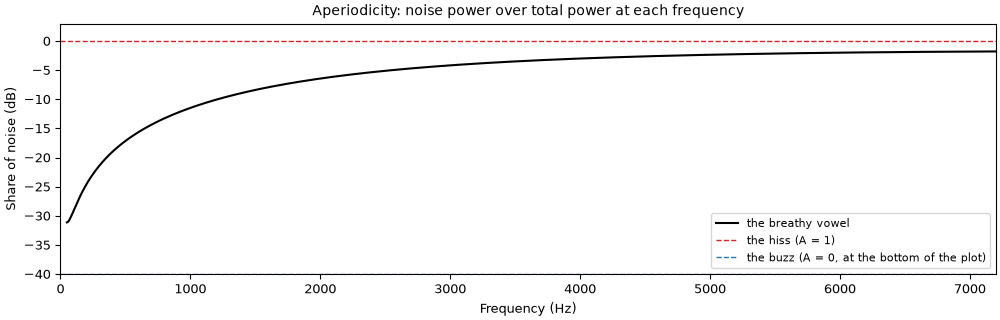
harmonics fall about 6 dB per octave and the noise is flat, so the share of noise rises about
6 dB per octave. Its level is set so that noise and harmonics are equally strong at 4 kHz.
Everything about the vowel is known, so its aperiodicity can be written down.
Code
import matplotlib.pyplot as plt
import numpy as np

import sonore as so

plt.rcParams.update({"font.size": 9, "axes.titlesize": 10, "figure.dpi": 100})
FS = 16000
F0 = 115.0
DUR = 1.0
HOD = [(730, 60), (1090, 90), (2440, 150), (3500, 200), (4500, 250)]


def finish(snd):
    """How every sound in the gallery is played: 5 ms ramps, RMS 0.1, peak at most 0.95."""
    snd = snd.ramp(5e-3).normalize(rms=0.1)
    return snd.normalize(peak=0.95) if snd.peak > 0.95 else snd


def show(snd, title, fmax=5000):
    """Waveform and narrowband spectrogram (Hann 33 ms, harmonics resolved), on one time axis."""
    fig = plt.figure(figsize=(10, 4.2), layout="constrained")
    ax0, ax1 = fig.subplots(2, 1, sharex=True, height_ratios=[0.45, 1])
    snd.plot(ax0, color="k", lw=0.4)
    ax0.set(title=f"Waveform: {title}", xlabel="")
    so.STFT(snd, win_dur=0.0333, hop_dur=0.002).plot(ax1, db_range=70, colorbar=False, fmax=fmax)
    ax1.set_title("Spectrogram (Hann 33 ms)")
    for ax in (ax0, ax1):
        ax.set_xlim(0, snd.duration)
    return fig, [ax0, ax1]


def formants(snd):
    for freq, bandwidth in HOD:
        snd = so.resonator(snd, freq, bandwidth)
    return snd


# Klatt's glottal source (an impulse through a low-pass resonator at 0 Hz, 100 Hz wide) and the
# radiation from the lips (a first difference), as a gain at any frequency.
impulse = so.Sound(np.r_[1.0, np.zeros(2**14 - 1)], FS)
glottal_gain = np.abs(np.fft.rfft(so.resonator(impulse, 0, 100).data[:, 0]))
gain_freqs = np.fft.rfftfreq(2**14, 1 / FS)


def source_gain(f):
    return np.interp(f, gain_freqs, glottal_gain) * np.abs(2 * np.sin(np.pi * np.asarray(f) / FS))


harmonic_numbers = np.arange(1, int(0.45 * FS / F0) + 1)
buzz = so.harmonic_complex(DUR, FS, F0, harmonics=harmonic_numbers, amplitudes=lambda t, f: source_gain(f))
# harmonic_complex scales its output to RMS 1; the harmonics' power per hertz near f is then
# (scale * gain(f))^2 / 2 per harmonic, one harmonic every F0 hertz
scale = 1 / np.sqrt(np.sum(source_gain(harmonic_numbers * F0) ** 2) / 2)


def harmonic_density(f):
    return (scale * source_gain(f)) ** 2 / 2 / F0


noise_density = harmonic_density(4000.0)  # noise as strong as the harmonics at 4 kHz
hiss = so.gaussian_noise(DUR, FS, rng=1) * np.sqrt(noise_density * FS / 2)  # white: flat density


def true_aperiodicity(f):
    """The share of noise at f, from the source alone."""
    return noise_density / (noise_density + harmonic_density(f))


vowel = formants(buzz + hiss)
window_times = np.arange(0, DUR, 0.005)
track = (window_times, np.full(len(window_times), F0))  # the exact F0, every 5 ms
inside = (window_times > 0.1) & (window_times < 0.9)  # time windows away from the ends
Buzz, hiss, and both
The first-order picture has two settings of the source, and the voice in between.
The buzz alone
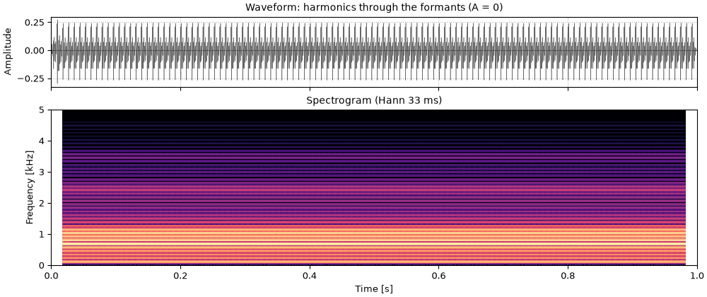
The buzz alone: harmonics through the formants, A = 0 everywhere. Every frequency is
periodic: the spectrogram shows harmonics all the way up, with nothing between them.
ap1_the_buzz_alone.flac, 1.0 s, mono
Code
sound = finish(formants(buzz))
fig, playhead = show(sound, "harmonics through the formants (A = 0)")
The hiss alone
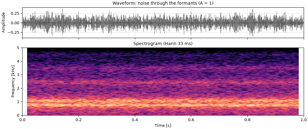
The hiss alone: white noise through the same formants, A = 1 everywhere. The vowel is still
there, whispered, because the formants are.
ap2_the_hiss_alone.flac, 1.0 s, mono
Code
sound = finish(formants(hiss))
fig, playhead = show(sound, "noise through the formants (A = 1)")
A breathy vowel
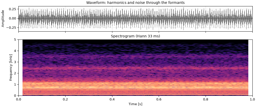
Both together. Below about 1 kHz the harmonics stand well above the noise; above 3 kHz the
noise fills in between them and then covers them. This is what makes a voice breathy: neither
switch setting, but a mixture whose proportion changes with frequency.
ap3_a_breathy_vowel.flac, 1.0 s, mono
Code
sound = finish(vowel)
fig, playhead = show(sound, "harmonics and noise through the formants")
Its aperiodicity is the noise's share of the source at each frequency. The harmonics and the
noise both pass through the same filter H, so the share after it is
the filter cancels. The aperiodicity is a property of the source, measured on the output,
and it can be changed without touching the formants, and the formants without touching it.
Aperiodicity of the vowel, from its source
Code
freqs = np.linspace(50, 7200, 1000)
fig, ax = plt.subplots(figsize=(10, 3.2), layout="constrained")
ax.plot(freqs, 10 * np.log10(true_aperiodicity(freqs)), color="k", label="the breathy vowel")
ax.axhline(0, color="C3", ls="--", lw=1, label="the hiss (A = 1)")
ax.axhline(-40, color="C0", ls="--", lw=1, label="the buzz (A = 0, at the bottom of the plot)")
ax.set(xlabel="Frequency (Hz)", ylabel="Share of noise (dB)", xlim=(0, 7200), ylim=(-40, 3))
ax.set_title("Aperiodicity: noise power over total power at each frequency")
ax.legend(loc="lower right", fontsize=8)
Fit the harmonics, keep the rest
The definition suggests the measurement: find the best periodic sound, take it away, and see
how much is left. If the pitch is known, the periodic part of a short stretch is a sum of
harmonics whose phases follow the running phase \Phi(t) = 2\pi \int F_0, each with an amplitude
and a phase to be found. That is a linear least-squares fit. Here is one time window, under a Hann
window four periods long, with each harmonic also allowed an amplitude that changes linearly
across the window.
Code
centre = int(0.5 * FS)  # the time window at 0.5 s
half = int(round(2 * FS / F0))  # half of four periods
offsets = np.arange(-half, half + 1)
window = 0.5 + 0.5 * np.cos(np.pi * offsets / (half + 1))
phase = 2 * np.pi * F0 * offsets / FS  # the running phase over the time window
harmonic_phases = np.outer(phase, np.arange(1, int(FS / 2 / F0) + 1))
ramp = (offsets / half)[:, None]
columns = np.column_stack(
    [np.ones(len(offsets)), np.cos(harmonic_phases), np.sin(harmonic_phases)]
    + [ramp * np.cos(harmonic_phases), ramp * np.sin(harmonic_phases)]
)
segment = vowel.data[centre + offsets, 0]
root_window = np.sqrt(window)  # weighted least squares: minimise the windowed residual
weights, *_ = np.linalg.lstsq(columns * root_window[:, None], segment * root_window, rcond=None)
residual = segment - columns @ weights
print(f"{columns.shape[1]} columns fitted to {len(offsets)} samples")
residual_power, signal_power = np.sum((window * residual) ** 2), np.sum((window * segment) ** 2)
print(f"windowed residual power over windowed signal power: {residual_power / signal_power:.3f}")
277 columns fitted to 557 samples
windowed residual power over windowed signal power: 0.012
One time window, before and after the harmonics are taken away
The time window's spectrum, and the spectrum of what is left after the fit. The harmonic peaks are
gone from the residual, and what remains is the noise between and under them. Where the noise
was below the harmonics (low frequencies) the residual lies far below the time window's spectrum;
above 4 kHz the two are close. Their ratio, read across frequency, is the aperiodicity.
Code
n_fft = 4096
segment_freqs = np.fft.rfftfreq(n_fft, 1 / FS)
segment_db = 20 * np.log10(np.abs(np.fft.rfft(window * segment, n_fft)) + 1e-12)
residual_db = 20 * np.log10(np.abs(np.fft.rfft(window * residual, n_fft)) + 1e-12)
fig, ax = plt.subplots(figsize=(10, 3.4), layout="constrained")
ax.plot(segment_freqs, segment_db, color="0.6", lw=0.7, label="the time window")
ax.plot(segment_freqs, residual_db, color="C3", lw=0.7, label="the time window less the fitted harmonics")
top = segment_db.max() + 5
ax.set(xlabel="Frequency (Hz)", ylabel="Level (dB)", xlim=(0, 6000), ylim=(top - 95, top))
ax.set_title("One time window of the breathy vowel (Hann, four periods)")
ax.legend(loc="upper right", fontsize=8)
so.harmonic_aperiodicity does this at every time window. It adds one correction: the fit also
absorbs a little of the noise, the part that happens to look like the harmonics near each
harmonic frequency, so the residual is a little too small there. How much is known exactly from
the fit itself (it is what the fit would do to white noise), and is divided out. The shares are
then summed over cells two harmonics wide and put on the frequency grid of WORLD's envelope.
The measure is the definition, which makes it easy to explain and to check. It has one
weakness: it needs the pitch to about a tenth of a percent. A harmonic whose frequency is
slightly wrong drifts out of phase with the fit over the window, and what the fit misses reads
as noise, more so the higher the harmonic. For the same reason it reads cycle-to-cycle
irregularity (jitter and shimmer) as noise.
What WORLD reports
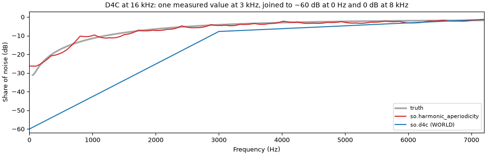
WORLD's own measure is D4C (Morise, 2016), which so.d4c reproduces exactly. It works from a
"group delay" of the time window, smoothed over the harmonics, whose spectrum is sorted to see how
much of its power lies outside the strongest components, in bands 3 kHz wide around each
multiple of 3 kHz. A correction for F0 follows, and the curve is drawn as straight lines (in dB)
from −60 dB at 0 Hz through the bands' values to 0 dB at the top. At 16 kHz there is only one
band, at 3 kHz. D4C's paper says it was tuned with listening tests so that WORLD's resynthesis
sounds natural; the −60 dB at 0 Hz says "the lowest frequencies are periodic", which is usually
true of speech.
D4C and the harmonic residual against the truth
Code
d4c_share = so.d4c(vowel, track)
fig, ax = plt.subplots(figsize=(10, 3.2), layout="constrained")
ax.plot(freqs, 10 * np.log10(true_aperiodicity(freqs)), color="k", lw=2.5, alpha=0.35, label="truth")
ax.plot(residual_share.f, 10 * np.log10(measured.mean(axis=1)), color="C3", label="so.harmonic_aperiodicity")
d4c_mean = d4c_share.share[0][:, inside].mean(axis=1)
ax.plot(d4c_share.f, 10 * np.log10(d4c_mean), color="C0", label="so.d4c (WORLD)")
ax.set(xlabel="Frequency (Hz)", ylabel="Share of noise (dB)", xlim=(0, 7200), ylim=(-62, 3))
ax.set_title("D4C at 16 kHz: one measured value at 3 kHz, joined to −60 dB at 0 Hz and 0 dB at 8 kHz")
ax.legend(loc="lower right", fontsize=8)
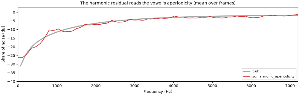
So the two answer different questions. The harmonic residual reports the share of noise. D4C
reports a value that makes WORLD's synthesis sound natural, and below 3 kHz it is far from
the share of noise on this vowel. In exchange, D4C hardly cares whether the pitch is exact.
Averaged over bands and time windows, with the exact pitch track and with one 1% too high:
Code
band_edges = [0, 1000, 2000, 4000, 7000]
envelope = so.cheaptrick(vowel, track)
# the truth in each band: noise power over total power, the envelope weighting each frequency
# as .bands() weights it
weights = envelope.data[0][:, inside].mean(axis=1)
truth_db = []
for low, high in zip(band_edges[:-1], band_edges[1:], strict=True):
    in_band = (envelope.f >= low) & (envelope.f < high)
    share = np.sum(true_aperiodicity(envelope.f[in_band]) * weights[in_band]) / np.sum(weights[in_band])
    truth_db.append(10 * np.log10(share))
wrong_track = (window_times, track[1] * 1.01)
bands = "".join(f"{f'{low}-{high}':>11}" for low, high in zip(band_edges[:-1], band_edges[1:], strict=True))
print(f"{'Share of noise [dB], band [Hz]':<34}{bands}")
print(f"{'truth':<34}" + "".join(f"{value:>11.1f}" for value in truth_db))
for name, measure in [("harmonic residual", so.harmonic_aperiodicity), ("D4C", so.d4c)]:
    for label, f0 in [("exact F0", track), ("F0 1% high", wrong_track)]:
        shares = measure(vowel, f0).bands(band_edges, envelope)[0][:, inside].mean(axis=1)
        print(f"{name + ', ' + label:<34}" + "".join(f"{value:>11.1f}" for value in 10 * np.log10(shares)))
Share of noise [dB], band [Hz]         0-1000  1000-2000  2000-4000  4000-7000
truth                                   -13.7      -10.8       -5.2       -2.8
harmonic residual, exact F0             -13.4      -10.4       -5.5       -3.1
harmonic residual, F0 1% high           -13.4       -9.3       -2.9       -0.2
D4C, exact F0                           -47.5      -40.8      -15.1       -5.7
D4C, F0 1% high                         -47.4      -40.8      -15.0       -5.7
With the wrong pitch, the harmonic residual's upper bands move toward 0 dB (all noise), as the
high harmonics drift out of phase with the fit; D4C's numbers do not change.
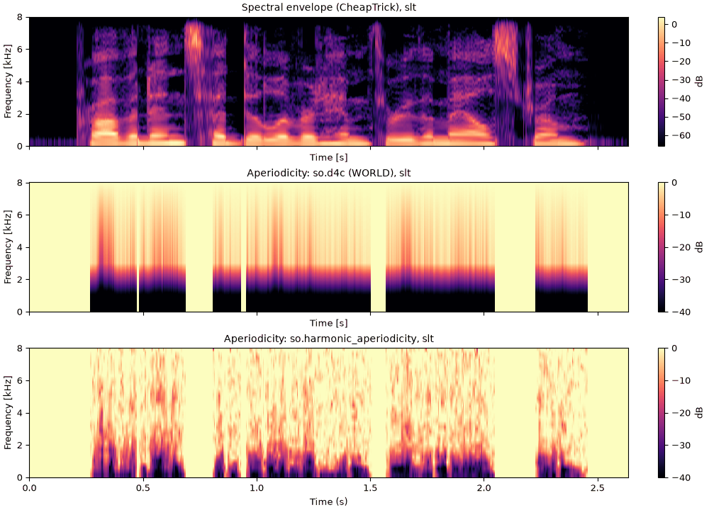
A sentence
The sentence from Seeing speech, with the F0 track WORLD's Harvest (Morise, 2017)
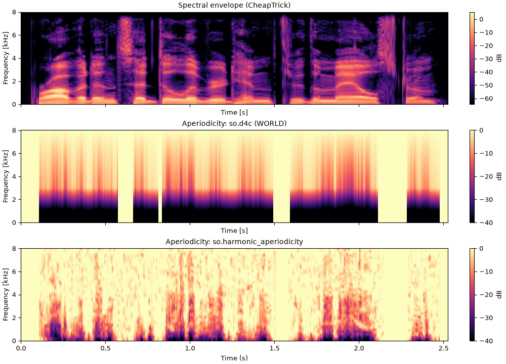
measured, stored with it. On recorded speech there is no truth to compare with, but the two
maps can be set side by side. Both are 1 (0 dB, all noise) where the track says unvoiced. In
voiced time windows the harmonic residual is low below 1 to 2 kHz, where the harmonics are strong,
and near 0 dB above about 4 kHz in many time windows; D4C has the same shape in every voiced time window,
a single bend at 3 kHz.
fig, axes = plt.subplots(3, 1, figsize=(10, 7.2), sharex=True, layout="constrained")
sentence_envelope.plot(axes[0], db_range=70)
axes[0].set_title("Spectral envelope (CheapTrick)")
for ax, aperiodicity, title in [
    (axes[1], sentence_d4c, "Aperiodicity: so.d4c (WORLD)"),
    (axes[2], sentence_residual, "Aperiodicity: so.harmonic_aperiodicity"),
]:
    aperiodicity.plot(ax, db_range=40)
    ax.set_title(title)
for ax in axes:
    ax.set_xlim(0, sentence.duration)
axes[2].set_xlabel("Time (s)")
Listening
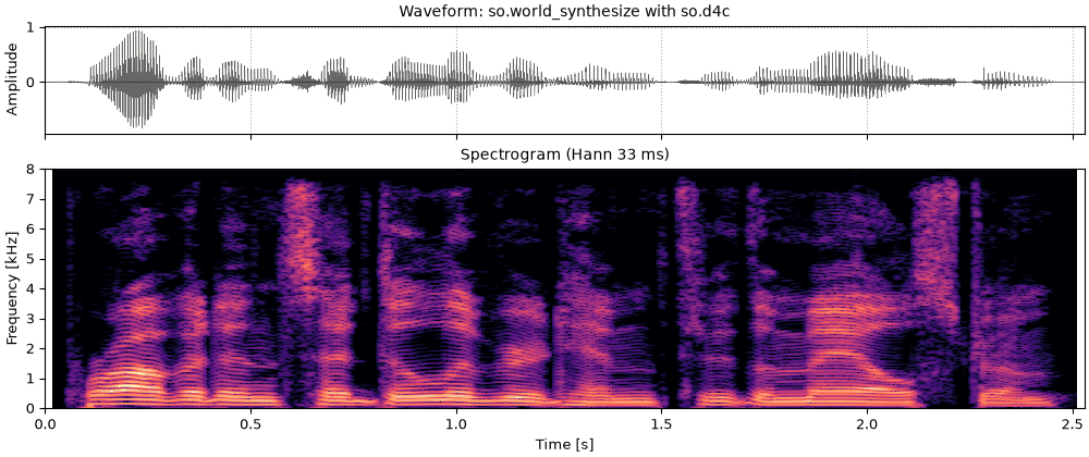
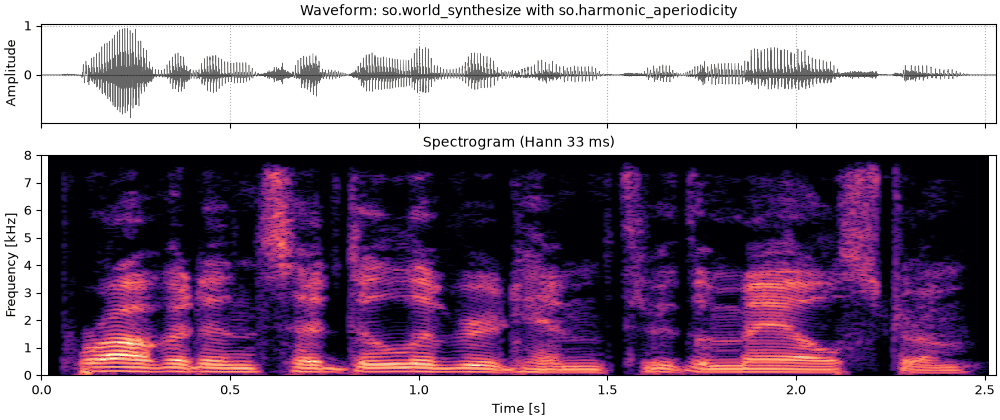
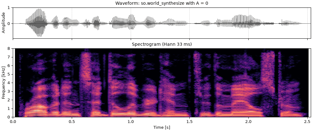
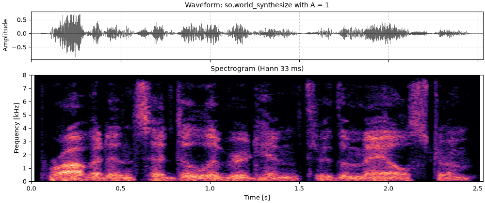
so.world_synthesize is WORLD's synthesis, reproduced sample for sample. At every pitch period
it adds two pieces: the harmonics' share of the envelope, S(1 - A), as one pulse, and the
noise's share, S A, as a short burst of filtered noise. Below, the same pitch track and
envelope with four aperiodicities. (WORLD keeps A between −60 dB and just under 0 dB, and
time windows the track calls unvoiced are always noise.)
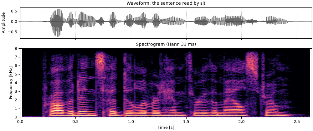
The sentence
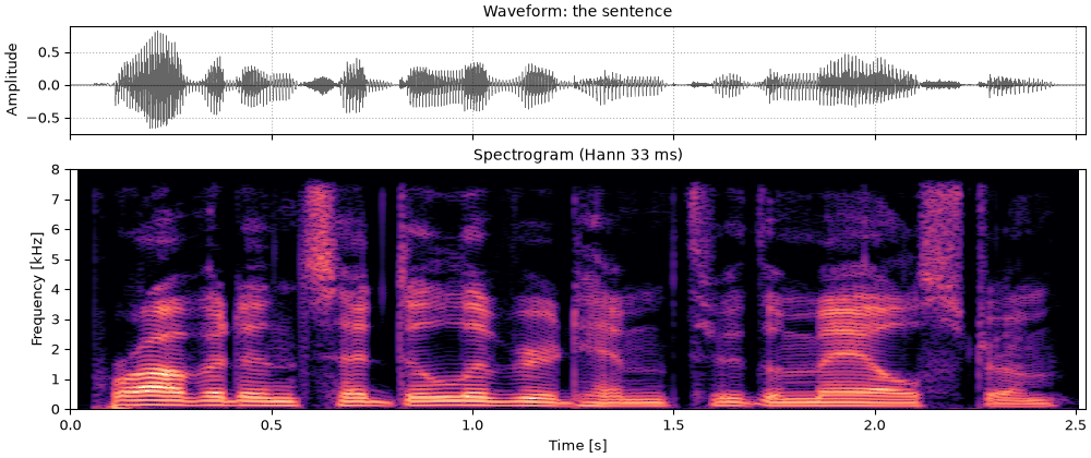
The sentence, for reference.
ap9_the_sentence.flac, 2.5 s, mono
Code
sound = sentence
fig, playhead = show(sound, "the sentence", fmax=8000)
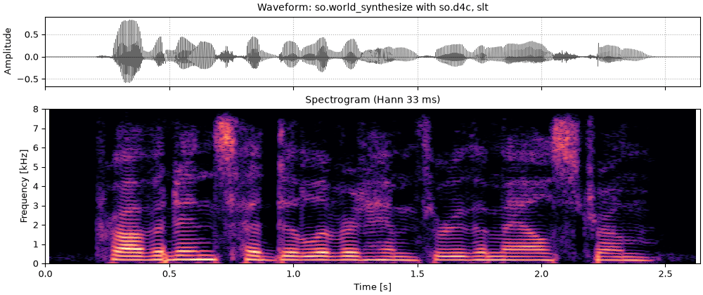
Resynthesis with D4C
WORLD's resynthesis, with D4C's aperiodicity: what WORLD itself makes from this pitch track,
sample for sample.
With A = 1 everywhere: noise only, through the same envelope. The pitch is gone and the
sentence is whispered; it is still intelligible, because the envelope carries the words.
ap13_nothing_but_noise.flac, 2.5 s, mono
Code
noise_only = so.Aperiodicity(np.ones_like(sentence_d4c.data), sentence_d4c.t, FS, "all noise")
sound = finish(so.world_synthesize(harvest, sentence_envelope, noise_only))
fig, playhead = show(sound, "so.world_synthesize with A = 1", fmax=8000)
A higher voice
Female voices sit about half an octave to an octave above male ones, so their harmonics are
further apart, and both measures have fewer of them to work with. The breathy vowel again,
made the same way but at 230 Hz, twice the pitch, with female formants for "hod" (average
F1 to F3 from Hillenbrand et al., 1995). The noise is again as strong as the harmonics at 4 kHz,
so the truth has the same shape as before.
harmonics below 7.2 kHz: 62 at 115 Hz, 31 at 230 Hz
Both measures at twice the pitch
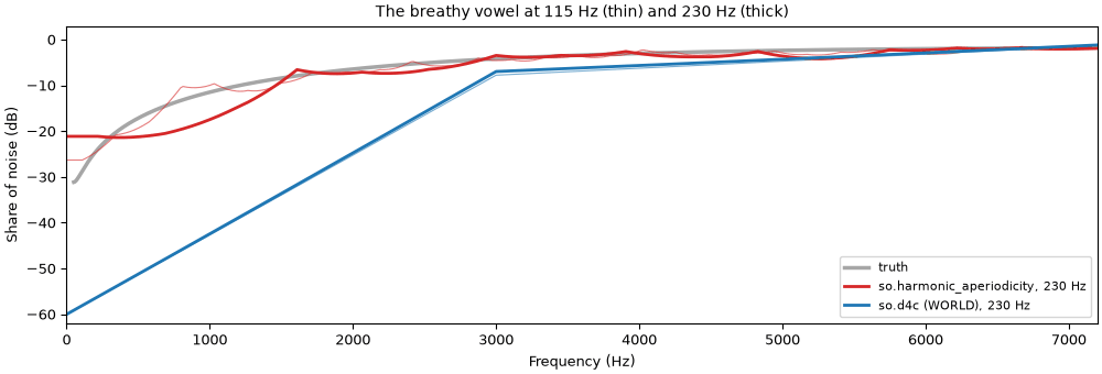
Both measures at 115 Hz (thin lines, as above) and at 230 Hz (thick lines), against the truth,
which is the same at both pitches. The harmonic residual fits half as many harmonics at the
higher pitch, in a window four of its shorter periods long; D4C's single band at 3 kHz gets a
different F0 correction.
truth_high_db = []
envelope_high = so.cheaptrick(vowel_high, track_high)
weights_high = envelope_high.data[0][:, inside].mean(axis=1)
for low, high in zip(band_edges[:-1], band_edges[1:], strict=True):
    in_band = (envelope_high.f >= low) & (envelope_high.f < high)
    share = np.sum(true_aperiodicity(envelope_high.f[in_band]) * weights_high[in_band]) / np.sum(
        weights_high[in_band]
    )
    truth_high_db.append(10 * np.log10(share))
print(f"{'Share of noise [dB], band [Hz]':<34}{bands}")
print(f"{'truth':<34}" + "".join(f"{value:>11.1f}" for value in truth_high_db))
for name, measure in [("harmonic residual", so.harmonic_aperiodicity), ("D4C", so.d4c)]:
    shares = measure(vowel_high, track_high).bands(band_edges, envelope_high)[0][:, inside].mean(axis=1)
    print(
        f"{name + f', {F0_HIGH:.0f} Hz':<34}" + "".join(f"{value:>11.1f}" for value in 10 * np.log10(shares))
    )
Share of noise [dB], band [Hz]         0-1000  1000-2000  2000-4000  4000-7000
truth                                   -12.3       -9.7       -4.7       -2.8
harmonic residual, 230 Hz               -18.6      -11.5       -5.4       -3.5
D4C, 230 Hz                             -44.2      -35.5      -10.8       -5.3
The same sentence read by a female talker (CMU ARCTIC, speaker slt). There is no stored Harvest
track for this recording, so the pitch comes from so.f0_track; the analysis is still WORLD's.
WORLD's pitch tracker. Harvest is not part of sonore; its track is stored with the sentence. With so.f0_track instead, the analysis is still WORLD's but the numbers are not the ones WORLD would give, which so.DIFFERENCES_FROM_WORLD notes.
Phase. WORLD's synthesis gives every pulse a minimum phase, so the waveform within each period is not the original's. Its authors call minimum phase inappropriate for low-pitched speech, where differences of phase are easier to hear.
Jitter and shimmer. A pitch track smoothed over 5 ms time windows cannot follow cycle-to-cycle irregularity, so the harmonic residual counts it as noise, and a resynthesis can only carry it as noise.
References
Hillenbrand, Getty, Clark & Wheeler (1995). Acoustic characteristics of American English vowels. J. Acoust. Soc. Am. 97(5), 3099–3111. doi:10.1121/1.411872. Female formants for "hod".
Klatt (1980). Software for a cascade/parallel formant synthesizer. J. Acoust. Soc. Am. 67(3), 971–995. doi:10.1121/1.383940. The glottal source.
Kominek & Black (2004). The CMU Arctic speech databases. Proc. 5th ISCA Speech Synthesis Workshop, 223–224. ISCA Archive. The sentence, by speakers bdl and slt.
Morise (2017). Harvest: a high-performance fundamental frequency estimator from speech signals. Proc. Interspeech 2017, 2321–2325. doi:10.21437/Interspeech.2017-68. The stored F0 track.
Morise, Yokomori & Ozawa (2016). WORLD: a vocoder-based high-quality speech synthesis system for real-time applications. IEICE Trans. Inf. & Syst. E99-D(7), 1877–1884. doi:10.1587/transinf.2015EDP7457. world.world_synthesize