Timbre

Timbre is usually defined by what it is not: whatever still tells two sounds apart when they have the same pitch, the same loudness and the same duration. A clarinet and a violin playing the same note differ in timbre, and so do two vowels sung on the same note. Grey (1977) made the first timbre space: listeners rated how different pairs of 16 resynthesized instrument tones sounded, and multidimensional scaling placed the tones in a space of three dimensions. Later spaces of the same kind (McAdams et al., 1995) had dimensions that correlated with three measurable properties of the sound: how fast it starts, how bright it is, and how much its spectrum changes. This page plays synthetic tones that move along one of those at a time, and measures each with sonore's timbre descriptors.

Press play and a line follows the sound across every time axis in its plots. Click any time axis to play from that point. Start with your volume low.

Code the examples share

Every tone is at E♭4 (311 Hz), the pitch of Grey (1977) and McAdams et al. (1995), and is a harmonic complex of 20 partials with amplitudes n^{-s} for harmonic n: the larger the slope s, the faster the partials fall and the duller the tone. Each partial rises linearly over its attack time and fades out over the last 100 ms. Tones are 1 s long, half a second apart, and set to the same RMS level. Equal RMS is not equal loudness: sonore has no loudness model, and a bright tone at the same RMS as a dull one usually sounds louder.

The three descriptors are those of Peeters et al. (2011), written from the paper's equations (docs/design/music/timbre-page.md says where sonore's defaults differ from the paper's, and why):

  • Log attack time (so.log_attack_time): \log_{10} of the attack's duration in seconds. The attack is found on the energy envelope (the amplitude of the signal, smoothed by a 20 Hz low-pass filter) by the paper's "weakest effort" method, which looks for where the envelope climbs fastest from one tenth of its maximum to the next. so.attack_segment gives its start and end.
  • Spectral centroid (so.spectral_centroid): the centre of gravity of the power spectrum, \sum_k f_k p_k / \sum_k p_k, in each 23.2 ms time window, every 5.8 ms. Its median over the tone is the usual measure of brightness.
  • Spectral flux (so.spectral_flux): one minus the correlation of two magnitude spectra 100 ms apart, 0 when the spectrum keeps its shape.

Each sound is drawn as a spectrogram with its centroid track over it and, under it, the waveform with each tone's measured attack shaded. Every sound starts with half a second of silence.

Code
import matplotlib.pyplot as plt
import numpy as np

import sonore as so

plt.rcParams.update({"font.size": 9, "axes.titlesize": 10, "figure.dpi": 100})
FS = 44100
F0 = so.note_to_freq("Eb4")
DUR = 1.0  # every tone [s]
GAP = 0.5  # silence before and between tones [s]
RELEASE = 0.1  # fade at the end of every tone [s]
HARMONICS = np.arange(1, 21)


def envelope(t, attack, duration=DUR):
    """A linear rise over ``attack`` seconds and a raised-cosine fade over the last RELEASE."""
    fade = 0.5 - 0.5 * np.cos(np.pi * np.clip((duration - t) / RELEASE, 0, 1))
    return np.minimum(1, t / attack) * fade


def tone(slope=1.0, attack=20e-3, duration=DUR):
    """E-flat 4 with 20 harmonics of amplitude n^-slope. ``slope`` may be a function of time
    and ``attack`` (the linear rise of each partial, in seconds) a function of the harmonic
    number."""

    def gain(t, f, n):
        s = slope(t) if callable(slope) else slope
        rise = attack(n) if callable(attack) else attack
        power = (HARMONICS[:, None] ** (-2.0 * np.asarray(s))).sum(0)  # keeps the level steady
        return float(n) ** -s / np.sqrt(power) * envelope(t, rise, duration)

    return so.harmonic_complex(duration, FS, F0, harmonics=HARMONICS, amplitudes=gain)


def finish(snd):
    """How every sound in the gallery is played: 5 ms ramps, RMS 0.1, peak at most 0.95."""
    snd = snd.ramp(5e-3).normalize(rms=0.1)
    return snd.normalize(peak=0.95) if snd.peak > 0.95 else snd


def describe(snd):
    """Log attack time, median centroid [Hz] and median flux of one tone."""
    return (
        so.log_attack_time(snd),
        so.spectral_centroid(snd).median[0],
        so.spectral_flux(snd).median[0],
    )


def sequence(tones):
    """The tones one after another, each at the same RMS, with GAP seconds before each one.
    Returns the sound and each tone's start time."""
    parts, starts, t = [], [], 0.0
    for snd in tones:
        parts += [so.silence(GAP, FS), snd.normalize(rms=0.1)]
        starts.append(t + GAP)
        t += GAP + snd.duration
    return finish(so.concat(parts + [so.silence(0.2, FS)])), starts


def show(snd, tones, starts, labels, fmin=150, fmax=8000, lower="envelope"):
    """Spectrogram with the centroid track, and under it the waveform with each tone's
    measured attack shaded (or, with ``lower="flux"``, the flux track). Returns the figure and the panels
    the playhead follows."""
    fig, (ax_s, ax_l) = plt.subplots(
        2, 1, figsize=(10, 5.4), sharex=True, height_ratios=[1.7, 1], layout="constrained"
    )
    stft = so.STFT(snd, 30e-3, 5e-3)
    keep = (stft.f >= fmin) & (stft.f <= fmax)
    level = stft.db[0][keep]
    ax_s.pcolormesh(stft.t, stft.f[keep], level, vmin=level.max() - 70, vmax=level.max(), cmap="magma")
    centroid = so.spectral_centroid(snd)
    ax_s.plot(centroid.t, centroid.values[0], color="c", lw=1.2, label="spectral centroid")
    ax_s.legend(loc="upper right", fontsize=8)
    ax_s.set(
        yscale="log",
        ylim=(fmin, fmax),
        ylabel="Frequency [Hz]",
        title="Spectrogram (Hann 30 ms) and spectral centroid (power)",
    )
    for start, label in zip(starts, labels, strict=True):
        ax_s.text(start + 0.02, 0.8 * fmax, label, color="w", fontsize=8, va="top")
    if lower == "flux":
        flux = so.spectral_flux(snd)
        ax_l.plot(flux.t, flux.values[0], color="C0")
        ax_l.set(yscale="log", ylim=(1e-5, 1), ylabel="Flux", title="Spectral flux, spectra 100 ms apart")
    else:
        t = np.arange(snd.n_samples) / FS
        ax_l.plot(t, np.abs(snd.data[:, 0]), color="0.75", lw=0.3)
        for start, snd_tone in zip(starts, tones, strict=True):
            begin, end = so.attack_segment(snd_tone)
            ax_l.axvspan(start + begin, start + end, color="C1", alpha=0.35, lw=0)
        ax_l.set(ylabel="Amplitude", title="Waveform magnitude, each measured attack shaded")
    ax_l.set(xlim=(0, snd.duration), xlabel="Time [s]")
    ax_l.grid(ls=":")
    return fig, [ax_s, ax_l]
Attack time

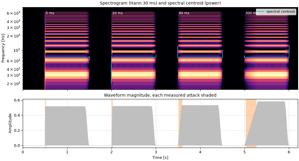
The same tone (s = 1) with its partials rising together over 5, 20, 80 and 300 ms. In McAdams et al. (1995) the first dimension of the timbre space correlated with the logarithm of the attack time, which is why it is measured on a log scale: 5 to 20 ms is as large a step as 80 to 320 ms. The cell prints each tone's true and measured attack.

Code
ATTACKS = [5e-3, 20e-3, 80e-3, 300e-3]
attack_tones = [tone(attack=attack) for attack in ATTACKS]
for attack, snd in zip(ATTACKS, attack_tones, strict=True):
    start, end = so.attack_segment(snd)
    lat = so.log_attack_time(snd)
    print(
        f"attack {1000 * attack:3.0f} ms: measured {1000 * (end - start):5.1f} ms, log attack time {lat:+.2f}"
    )
attack   5 ms: measured  16.1 ms, log attack time -1.79
attack  20 ms: measured  24.5 ms, log attack time -1.61
attack  80 ms: measured  87.9 ms, log attack time -1.06
attack 300 ms: measured 240.8 ms, log attack time -0.62

The measure is not exact: the envelope has to be smoothed before the attack can be found, and the smoothing stretches short attacks and shortens long linear ones, whose last tenth the weakest-effort method leaves out. What matters for a timbre space is that the order and the steps come out right. The paper's own setting for its descriptors smooths with a 5 Hz filter, which measures the 5 ms attack as about 80 ms (so.log_attack_time(snd, cutoff=5, zero_phase=False)); sonore uses the 20 Hz filter the paper uses to find onsets.

Attacks of 5, 20, 80 and 300 ms

Four tones, attacks of 5, 20, 80 and 300 ms. The first starts with a click, the second is still crisp, the third is soft and the last swells in like a bowed or blown note. The spectrum is the same throughout, and so is the centroid once each tone has started.

tb1_attacks_of_5_20_80_and_300_ms.flac, 6.2 s, mono

Plots of the attacks of 5, 20, 80 and 300 ms sound
Code
sound, starts = sequence(attack_tones)
fig, playhead = show(sound, attack_tones, starts, [f"{1000 * a:.0f} ms" for a in ATTACKS])

Brightness

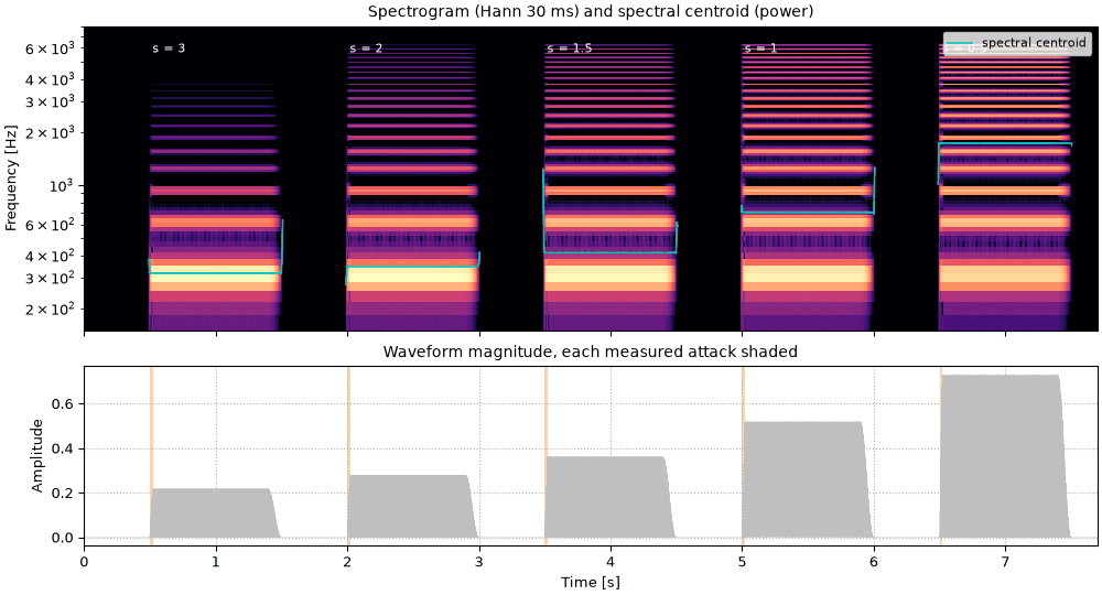
The second dimension of most timbre spaces follows the spectral centroid: where the energy sits on the frequency axis. Five tones with the same attack (20 ms) and the slope of their partials going from s = 3, where the fundamental dominates, to s = 0.5, where the high partials are almost as strong. The cell prints each one's median centroid over the power spectrum (the default), in hertz and in multiples of the fundamental, and over the magnitude spectrum.

Code
SLOPES = [3.0, 2.0, 1.5, 1.0, 0.5]
bright_tones = [tone(slope=slope) for slope in SLOPES]
for slope, snd in zip(SLOPES, bright_tones, strict=True):
    power = so.spectral_centroid(snd).median[0]
    magnitude = so.spectral_centroid(snd, scale="magnitude").median[0]
    ratio = power / F0
    print(
        f"slope {slope:3.1f}: power centroid {power:5.0f} Hz ({ratio:3.1f} x F0),"
        f" magnitude centroid {magnitude:4.0f} Hz"
    )
slope 3.0: power centroid   317 Hz (1.0 x F0), magnitude centroid  803 Hz
slope 2.0: power centroid   345 Hz (1.1 x F0), magnitude centroid  952 Hz
slope 1.5: power centroid   414 Hz (1.3 x F0), magnitude centroid 1237 Hz
slope 1.0: power centroid   701 Hz (2.3 x F0), magnitude centroid 1792 Hz
slope 0.5: power centroid  1730 Hz (5.6 x F0), magnitude centroid 2546 Hz

Which spectrum the centroid is taken over matters. Peeters et al. (2011) offer both, and for the same tone they can differ by a factor of more than two, so a centroid means little without saying which. The power centroid of a steady tone is exactly the one computed from its partials. The magnitude centroid weights weak components more, which spreads the dull tones further apart, but it also counts the window's sidelobes, small magnitudes spread over every frequency bin up to half the sample rate. For the s = 3 tone those outweigh the weak upper partials: its magnitude centroid is almost twice the 414 Hz its partials give, and would be lower at a lower sample rate (tools/check_timbre_claims.py).

Five tones from dull to bright

Five tones from dull to bright: slopes 3, 2, 1.5, 1 and 0.5. The pitch stays E♭4 while the centroid, the cyan line, climbs from the fundamental to about 1.7 kHz. The brightest tone is buzzy, brighter than a sawtooth wave, whose partials fall as 1/n.

tb2_five_tones_from_dull_to_bright.flac, 7.7 s, mono

Plots of the five tones from dull to bright sound
Code
sound, starts = sequence(bright_tones)
fig, playhead = show(sound, bright_tones, starts, [f"s = {s:g}" for s in SLOPES])

Spectral flux

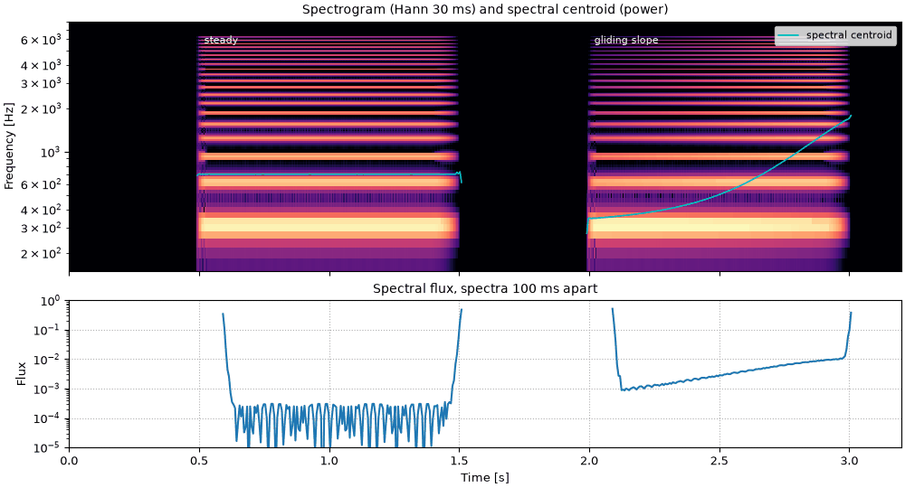
The third dimension in McAdams et al. (1995) correlated, more weakly, with spectral flux: how much the spectrum changes over the course of a tone. A steady tone (s = 1 throughout) is played next to one whose slope glides from 2 to 0.5 over its second, so that it starts dull and ends bright at a steady pitch and level. The cell prints the median flux of each, for spectra 100 ms apart and, as in the paper, for successive time windows 5.8 ms apart.

Code
steady = tone()
gliding = tone(slope=lambda t: 2.0 - 1.5 * t / DUR)
flux_tones = [steady, gliding]
for name, snd in zip(["steady", "gliding"], flux_tones, strict=True):
    apart = so.spectral_flux(snd).median[0]
    hop = so.spectral_flux(snd, spacing=None).median[0]
    print(f"{name:8s} flux x 1e6, 100 ms apart: {1e6 * apart:5.0f}, one time window apart: {1e6 * hop:4.0f}")
steady   flux x 1e6, 100 ms apart:   153, one time window apart:   91
gliding  flux x 1e6, 100 ms apart:  3272, one time window apart:  109

At 100 ms the gliding tone's flux is many times the steady one's; one time window apart the two are close, because a spectrum that changes slowly hardly changes in 5.8 ms. That is why sonore measures flux 100 ms apart by default (spacing=None gives the paper's version). Flux is the least settled of the three: published timbre spaces define it in several ways, and its correlation with the third dimension (0.54 in McAdams et al., 1995) is weaker than the other two (0.94 each).

A steady tone and a brightening one

A steady tone, then one that brightens over its second. The centroid of the second climbs steadily, and its flux, in the lower panel (on a logarithmic scale), stays about twenty times the steady tone's while it does. The spikes at the start and end of each tone are where one of the two spectra compared falls in the silence around it.

tb3_a_steady_tone_and_a_brightening_one.flac, 3.2 s, mono

Plots of the a steady tone and a brightening one sound
Code
sound, starts = sequence(flux_tones)
fig, playhead = show(sound, flux_tones, starts, ["steady", "gliding slope"], lower="flux")

Three descriptors at once

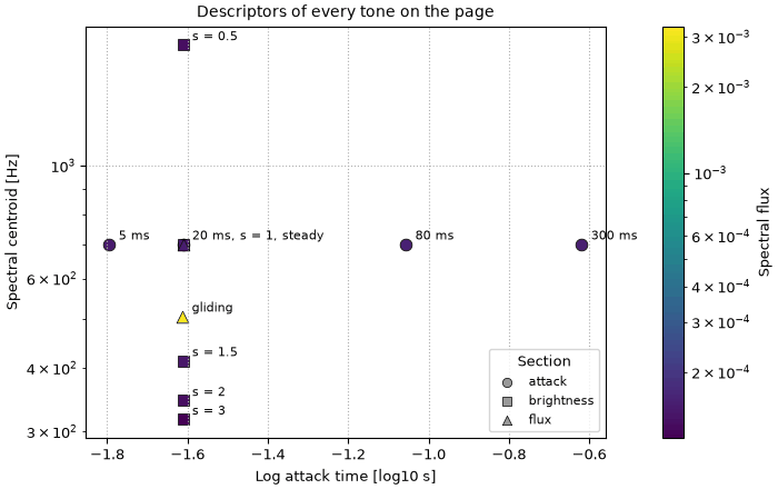
Every tone of the three sections above, placed by its three numbers: log attack time across, centroid up, and flux as the colour. The axes are descriptors computed from the sound, not a timbre space built from listeners' ratings; a timbre space would also say how much each axis counts, and might bend or merge them. Three of the points are one tone (the 20 ms attack, s = 1 and the steady tone), and the centroid axis is logarithmic.

Every tone of the page by its descriptors

Every tone of the page by its descriptors
Code
# the 20 ms attack, s = 1 and the steady tone are one tone, labelled once
groups = [
    ("attack", attack_tones, ["5 ms", "", "80 ms", "300 ms"], "o"),
    ("brightness", bright_tones, ["s = 3", "s = 2", "s = 1.5", "20 ms, s = 1, steady", "s = 0.5"], "s"),
    ("flux", flux_tones, ["", "gliding"], "^"),
]
points = [
    (name, label, marker, *describe(snd))
    for name, tones, labels, marker in groups
    for snd, label in zip(tones, labels, strict=True)
]
fluxes = np.array([p[5] for p in points])
fig, ax = plt.subplots(figsize=(7, 4.4), layout="constrained")
norm = plt.matplotlib.colors.LogNorm(fluxes.min(), fluxes.max())
for _, label, marker, lat, centroid, flux in points:
    ax.scatter(lat, centroid, c=[flux], cmap="viridis", norm=norm, marker=marker, s=60, edgecolor="k", lw=0.5)
    if label:
        ax.annotate(label, (lat, centroid), textcoords="offset points", xytext=(6, 3), fontsize=8)
for name, _, _, marker in groups:
    ax.scatter([], [], marker=marker, color="0.6", edgecolor="k", lw=0.5, label=name)
fig.colorbar(plt.cm.ScalarMappable(norm=norm, cmap="viridis"), ax=ax, label="Spectral flux")
ax.legend(title="Section", loc="lower right", fontsize=8)
ax.set(
    xlabel="Log attack time [log10 s]",
    ylabel="Spectral centroid [Hz]",
    title="Descriptors of every tone on the page",
)
ax.set_yscale("log")
ax.grid(ls=":")

Onsets

Much of what identifies an instrument is in the first moments of a note. Siedenburg (2019) played listeners 64 ms excerpts of ten instruments and asked them to name the instrument (chance was 10%). Excerpts from the onset were named 77% of the time, the same excerpts with the fast transient at the very start removed 71%, and excerpts from the middle of the tone 52%. So the onset matters, but mostly through the way the partials build up; the transient itself (a hammer's knock, a pipe's chiff) counted for less.

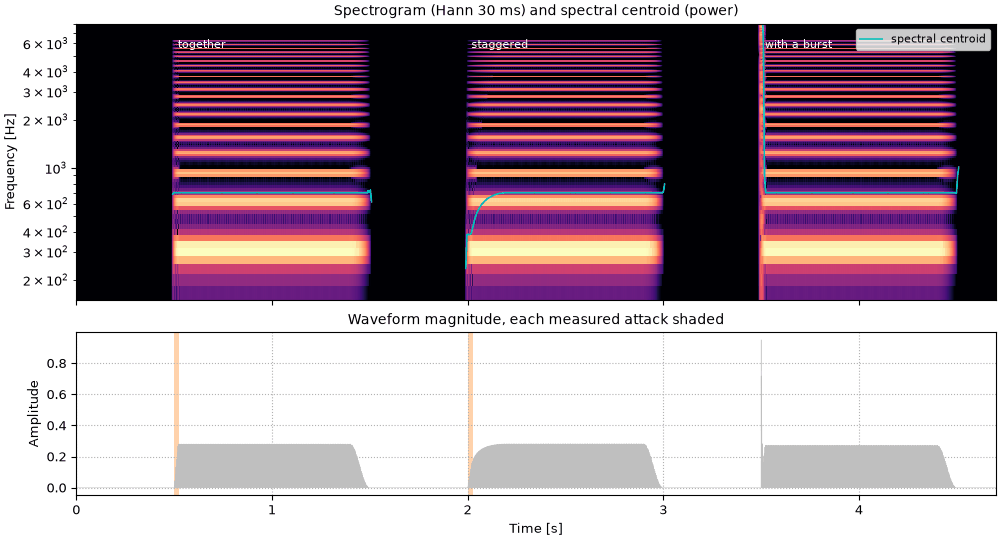
His sounds were recordings. Three synthetic versions of the idea, on one tone (s = 1): all partials starting together over 20 ms; the partials building up at different rates, from 20 ms for the fundamental to 200 ms for the 20th harmonic, as brass instruments do (an illustration, not a measured brass onset); and the first tone with a 15 ms burst of noise at its start, a stand-in for a transient. The cell prints the three descriptors of each, and the centroid over the first 100 ms alone.

Code
together = tone()
staggered = tone(attack=lambda n: 20e-3 + 180e-3 * (n - 1) / 19)
rng = np.random.default_rng(1)
burst_t = np.arange(int(15e-3 * FS)) / FS
burst = rng.standard_normal(len(burst_t)) * np.exp(-burst_t / 4e-3)
burst *= 2 * together.rms / np.sqrt(np.mean(burst**2))  # an estimate of a noticeable level
with_burst = so.Sound(together.data[:, 0] + np.pad(burst, (0, together.n_samples - len(burst))), FS)
onset_tones = [together, staggered, with_burst]
onset_labels = ["together", "staggered", "with a burst"]
for name, snd in zip(onset_labels, onset_tones, strict=True):
    lat, centroid, flux = describe(snd)
    early = so.spectral_centroid(so.Sound(snd.data[: int(0.1 * FS)], FS)).median[0]
    print(
        f"{name:13s} log attack {lat:+.2f}, centroid {centroid:5.0f} Hz (first 100 ms {early:5.0f} Hz),"
        f" flux {1e6 * flux:4.0f} x 1e-6"
    )
together      log attack -1.61, centroid   701 Hz (first 100 ms   701 Hz), flux  153 x 1e-6
staggered     log attack -1.59, centroid   701 Hz (first 100 ms   530 Hz), flux  240 x 1e-6
with a burst  log attack -2.72, centroid   701 Hz (first 100 ms   701 Hz), flux  153 x 1e-6

Three onsets of one tone

The same tone three times: partials starting together, the high partials arriving late, and a burst of noise added at the start. The second swells into brightness, which shows in the centroid line over its first fifth of a second; the third has a sharp tick at the start and is otherwise the first tone.

tb5_three_onsets_of_one_tone.flac, 4.7 s, mono

Plots of the three onsets of one tone sound
Code
sound, starts = sequence(onset_tones)
fig, playhead = show(sound, onset_tones, starts, onset_labels)

Summaries over a whole tone hide most of what happens in its first tenth of a second: the median centroids of the three are the same, while the centroid of the first 100 ms is lower for the staggered onset. The burst does the opposite to the log attack time: its peak is higher than the tone's, so the weakest-effort method finds the burst itself and measures an attack of a few milliseconds. A descriptor can weigh a transient far more than listeners did in Siedenburg's study, where removing it cost 6 points.

Vowels are timbres

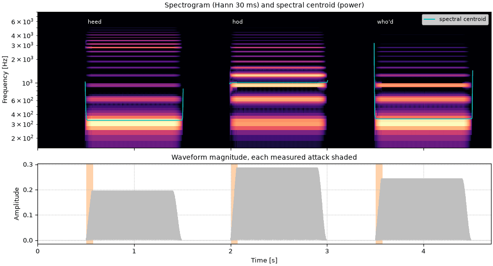
Two vowels sung on the same pitch and at the same level differ in their spectral envelopes: the formants, the resonances of the vocal tract, sit at different frequencies. In that sense different vowels are different timbres of one voice, and much of what the speech pages show applies here. Three vowels from so.klatt_synthesize, with Peterson and Barney's (1952) female formants for "heed", "hod" and "who'd", sung on E♭4 like the tones above, with the same envelope and RMS. Formant synthesis builds vowels from a source and a few resonances, and Cepstral analysis separates a voice's pitch from its spectral envelope, the part that carries the vowel.

Code
VOWELS = {"heed": (310, 2790, 3310), "hod": (850, 1220, 2810), "who'd": (370, 950, 2670)}
sung = envelope(np.arange(int(DUR * FS)) / FS, 60e-3)
vowel_tones = []
for f1, f2, f3 in VOWELS.values():
    voice = so.klatt_synthesize(DUR, FS, F0=F0, F1=f1, F2=f2, F3=f3, F4=4100, F5=4900)
    vowel_tones.append(voice * sung[:, None])
for word, snd in zip(VOWELS, vowel_tones, strict=True):
    print(f"{word:6s} centroid {so.spectral_centroid(snd).median[0]:5.0f} Hz")
heed   centroid   334 Hz
hod    centroid  1009 Hz
who'd  centroid   349 Hz

Three vowels on one note

"Heed", "hod" and "who'd" on one note. The harmonics are the same in all three, 311 Hz apart; only their strengths change. The centroid of "hod", whose first formant is high, is about three times that of the other two.

tb6_three_vowels_on_one_note.flac, 4.7 s, mono

Plots of the three vowels on one note sound
Code
sound, starts = sequence(vowel_tones)
fig, playhead = show(sound, vowel_tones, starts, list(VOWELS))

A centroid alone cannot tell vowels apart: "heed" and "who'd" sound nothing alike, yet their centroids are within a few percent of each other. Both have their first formant near the fundamental, which then dominates the power spectrum, and they differ in their second formant (2790 against 950 Hz), where the harmonics are much weaker. The formants, or a spectral envelope, describe vowels better than any one number, and the same is true of instruments.

References

  • Grey (1977). Multidimensional perceptual scaling of musical timbres. J. Acoust. Soc. Am. 61(5), 1270–1277. doi:10.1121/1.381428.
  • McAdams, Winsberg, Donnadieu, De Soete & Krimphoff (1995). Perceptual scaling of synthesized musical timbres: common dimensions, specificities, and latent subject classes. Psychol. Res. 58, 177–192. doi:10.1007/BF00419633.
  • Peeters, Giordano, Susini, Misdariis & McAdams (2011). The Timbre Toolbox: extracting audio descriptors from musical signals. J. Acoust. Soc. Am. 130(5), 2902–2916. doi:10.1121/1.3642604.
  • Peterson & Barney (1952). Control methods used in a study of the vowels. J. Acoust. Soc. Am. 24(2), 175–184. ASA.
  • Siedenburg (2019). Specifying the perceptual relevance of onset transients for musical instrument identification. J. Acoust. Soc. Am. 145(2), 1078–1087. doi:10.1121/1.5091778.