A voice is a source filtered by the vocal tract. In a formant synthesizer every part of that
sentence is a number: the source's pitch and level, and the frequency and bandwidth of each
resonance (formant). so.klatt_synthesize follows Klatt (1980). Voicing is a set of harmonics
of F_0 with the spectrum of Klatt's glottal pulse, aspiration and frication are noise, and
formants are second-order resonators
y[n] = A\,x[n] + B\,y[n-1] + C\,y[n-2],
with C = -e^{-2\pi B_k T}, B = 2e^{-\pi B_k T}\cos(2\pi F_k T) and A = 1 - B - C for a
formant at F_k Hz, B_k Hz wide, sampled every T seconds. Every parameter is a number or a
track of (times, values), so the sounds below are written down rather than recorded, and any
cue can be changed while the others stay put.
Press play and a line follows the sound across every time axis in its plots. Click any time
axis to play from that point. Start with your volume low.
Code the examples share
All the sounds are at 16 kHz. Each one is drawn as a waveform
and a wideband spectrogram (Hann 6 ms), which shows formants as dark bands, with the formant
frequencies the synthesizer was given drawn over it.
Code
import matplotlib.pyplot as plt
import numpy as np

import sonore as so

plt.rcParams.update({"font.size": 9, "axes.titlesize": 10, "figure.dpi": 100})
FS = 16000


def finish(snd):
    """How every sound in the gallery is played: 5 ms ramps, RMS 0.1, peak at most 0.95."""
    snd = snd.ramp(5e-3).normalize(rms=0.1)
    return snd.normalize(peak=0.95) if snd.peak > 0.95 else snd


def onoff(dur, level=60, on=0.02, off=0.05):
    """An amplitude track: up over `on` seconds, down over the last `off` seconds."""
    return ([0, on, dur - off, dur], [0, level, level, 0])


def show(snd, title, formants=()):
    """Waveform and wideband spectrogram, with formant tracks ((times, values) or numbers) drawn over it."""
    fig = plt.figure(figsize=(10, 4.2), layout="constrained")
    ax0, ax1 = fig.subplots(2, 1, sharex=True, height_ratios=[0.45, 1])
    snd.plot(ax0, color="k", lw=0.4)
    ax0.set(title=f"Waveform: {title}", xlabel="")
    frame = so.GaborFrame(0.006, 0.001, n_fft=512)  # zero-padded for smooth bands
    so.STFT(snd, frame=frame).plot(ax1, db_range=60, colorbar=False, fmax=5000)
    ax1.set_title("Spectrogram (Hann 6 ms), with the formant frequencies given to the synthesizer")
    for f in formants:
        t, v = ([0], [f]) if np.isscalar(f) else f  # a track is held after its last point
        ax1.plot([*t, snd.duration], np.array([*v, v[-1]]) / 1000, color="c", lw=1, ls="--")  # in kHz
    for ax in (ax0, ax1):
        ax.set_xlim(0, snd.duration)
    return fig, [ax0, ax1]
A vowel, piece by piece
The vowel of "hod", with Peterson and Barney's (1952) average male formants: 730, 1090 and
2440 Hz. The pitch falls from 130 to 100 Hz, as at the end of a statement. Here the pieces are
put together by hand with so.resonator, the same resonator so.klatt_synthesize uses.
Code
DUR = 1.0
F0 = ([0, DUR], [130, 100])
HOD = [(730, 60), (1090, 90), (2440, 150), (3500, 200), (4500, 250)]

# Klatt's glottal source: harmonics with the spectrum of an impulse through a low-pass
# resonator at 0 Hz, 100 Hz wide (about -12 dB per octave above 50 Hz).
glottal = so.Sound(np.r_[1.0, np.zeros(2**14 - 1)], FS)
rgp = np.abs(np.fft.rfft(so.resonator(glottal, 0, 100).data[:, 0]))
freqs = np.fft.rfftfreq(2**14, 1 / FS)
source = so.harmonic_complex(DUR, FS, F0, amplitudes=lambda t, f: np.interp(f, freqs, rgp))
# Radiation from the lips: a first difference, +6 dB per octave.
source = so.Sound(np.diff(source.data[:, 0], prepend=0.0), FS)
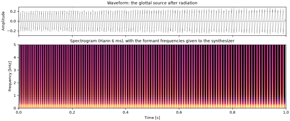
The source alone
The source on its own: the glottal pulse train after radiation, a buzz with no vowel in it.
Its harmonics fall smoothly with frequency, with no peaks.
fv1_the_source_alone.flac, 1.0 s, mono
Code
sound = finish(source)
fig, playhead = show(sound, "the glottal source after radiation")
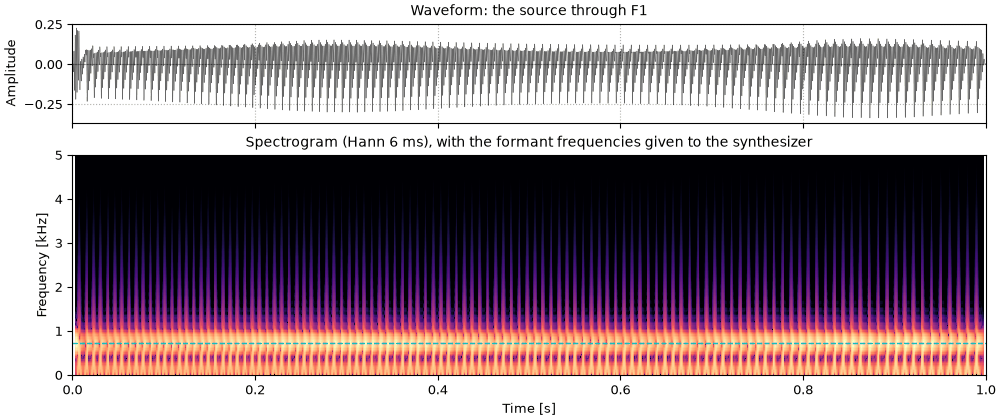
The first formant
Through the first formant only, at 730 Hz. The buzz becomes a dull, muffled vowel: all that is
left is energy around F1.
fv2_the_first_formant.flac, 1.0 s, mono
Code
one = so.resonator(source, *HOD[0])
sound = finish(one)
fig, playhead = show(sound, "the source through F1", [730])
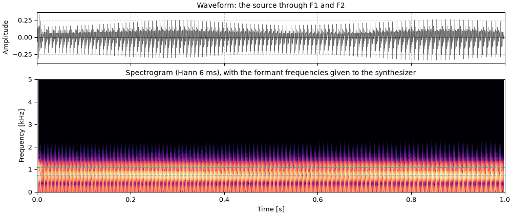
Two formants
Through the first two formants. F1 and F2 are what tells most vowels apart, and with both, the
sound is recognisably the vowel of "hod", if thin.
fv3_two_formants.flac, 1.0 s, mono
Code
two = so.resonator(one, *HOD[1])
sound = finish(two)
fig, playhead = show(sound, "the source through F1 and F2", [730, 1090])
Five formants
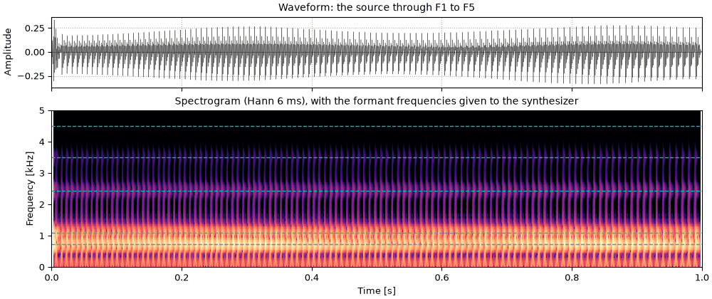
All five formants in cascade (one after the other). F3 to F5 add the brightness of a real
voice; their levels follow from their frequencies, as they do in a vocal tract.
fv4_five_formants.flac, 1.0 s, mono
Code
vowel = source
for f, bw in HOD:
    vowel = so.resonator(vowel, f, bw)
sound = finish(vowel)
fig, playhead = show(sound, "the source through F1 to F5", [f for f, _ in HOD])
The same vowel from so.klatt_synthesize
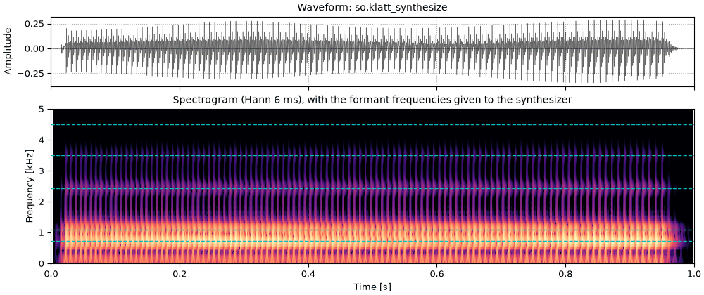
The same vowel from so.klatt_synthesize, with the voicing switched on and off over 20 and
50 ms. Apart from those ramps it is the sound above: the synthesizer does the same steps.
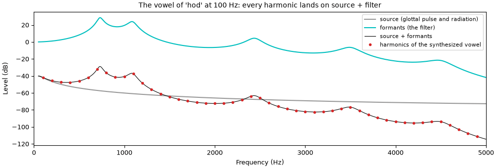
Because the source and the formants are separate, the spectrum of the vowel is the product of
their spectra: in dB, a sum. Here the pitch is held at 100 Hz, so the harmonics sit at
multiples of 100 Hz; each one's level is the source's level at that frequency plus the
formants' gain there.
The vowel spectrum as source plus filter
Code
vowel = so.klatt_synthesize(1.0, FS, F0=100, **hod)
spec = np.abs(np.fft.rfft(vowel.data[-FS // 2 :, 0]))  # the last 0.5 s, 2 Hz per bin
k = np.arange(1, 50)
measured = 20 * np.log10(spec[k * 50])  # harmonic k at 100 k Hz is bin 50 k
f = np.linspace(50, 5000, 2000)
z = np.exp(-2j * np.pi * f / FS)


def gain(fk, bk, f):
    c, b = -np.exp(-2 * np.pi * bk / FS), 2 * np.exp(-np.pi * bk / FS) * np.cos(2 * np.pi * fk / FS)
    zf = np.exp(-2j * np.pi * f / FS)
    return np.abs((1 - b - c) / (1 - b * zf - c * zf**2))


src_db = 20 * np.log10(gain(0, 100, f) * np.abs(1 - z))
filt_db = 20 * np.log10(np.prod([gain(fk, bk, f) for fk, bk in HOD], axis=0))
total = src_db + filt_db
harmonics = measured - measured[0] + np.interp(100, f, total)  # the output's level is arbitrary

fig, ax = plt.subplots(figsize=(10, 3.4), layout="constrained")
ax.plot(f, src_db, color="0.6", label="source (glottal pulse and radiation)")
ax.plot(f, filt_db, color="c", label="formants (the filter)")
ax.plot(f, total, color="k", lw=0.8, label="source + formants")
ax.plot(k * 100, harmonics, "o", ms=3, color="C3", label="harmonics of the synthesized vowel")
ax.set(xlabel="Frequency (Hz)", ylabel="Level (dB)", xlim=(0, 5000))
ax.set_title("The vowel of 'hod' at 100 Hz: every harmonic lands on source + filter")
ax.legend(loc="upper right", fontsize=8)
Six vowels
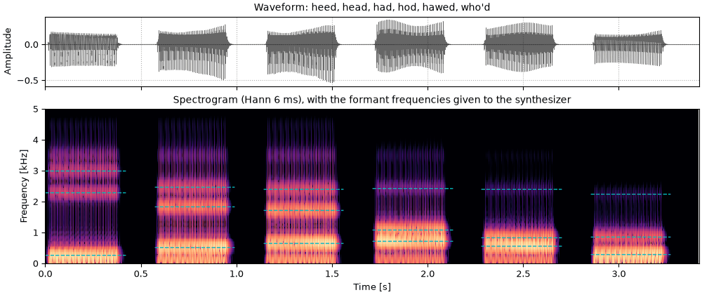
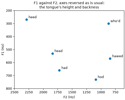
Peterson and Barney (1952) measured the formants of ten American English vowels, spoken in words
of the form h-vowel-d by male and female adults and by children. Their male averages, for six of
the vowels, synthesized with everything else the same: the pitch, the higher formants and the
bandwidths.
The six vowels in turn, from "heed" to "who'd". The dashed lines are each vowel's F1, F2 and F3.
fw1_six_vowels.flac, 3.4 s, mono
Code
sound = finish(so.concat(parts))
tracks = [
    (np.repeat(starts, 2) + np.tile([0, VOWEL_DUR], 6), np.repeat([v[i] for v in VOWELS.values()], 2))
    for i in range(3)
]
fig, playhead = show(sound, "heed, head, had, hod, hawed, who'd")
for tt, ff in tracks:
    for j in range(6):
        playhead[1].plot(tt[2 * j : 2 * j + 2], ff[2 * j : 2 * j + 2] / 1000, color="c", lw=1, ls="--")
The vowels by their first two formants
Code
fig, ax = plt.subplots(figsize=(5, 4), layout="constrained")
for word, (f1, f2, _) in VOWELS.items():
    ax.plot(f2, f1, "o", color="C0")
    ax.annotate(word, (f2, f1), textcoords="offset points", xytext=(6, 4))
ax.set(xlabel="F2 (Hz)", ylabel="F1 (Hz)", xlim=(2500, 600), ylim=(800, 200))
ax.set_title("F1 against F2, axes reversed as is usual:\nthe tongue's height and backness")
From heed to hod in seven steps
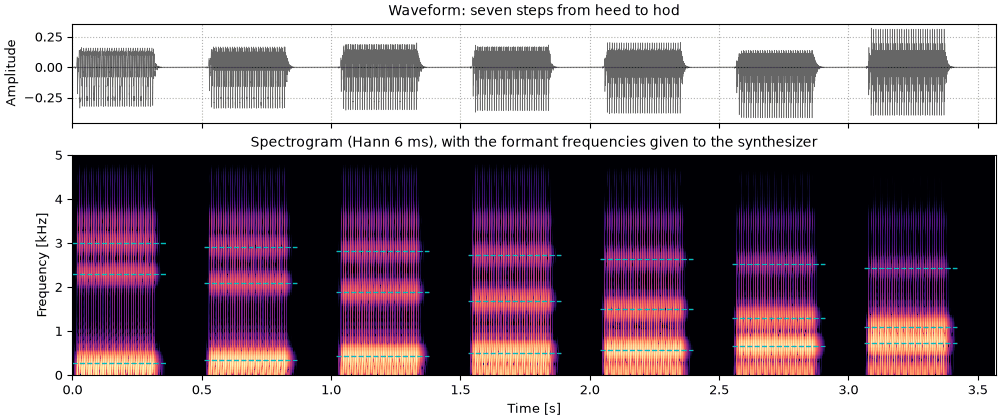
A continuum from "heed" to "hod" in seven equal steps of F1, F2 and F3, made with
so.klatt_continuum. Somewhere in the middle the vowel stops being one and becomes the
other; experiments on vowel categories use continua like this one.
steps = so.klatt_continuum(dict(F1=270, F2=2290, F3=3010), dict(F1=730, F2=1090, F3=2440), 7)
STEP_DUR = 0.36
parts = []
for p in steps:
    parts += [so.klatt_synthesize(STEP_DUR, FS, p, F0=110, AV=onoff(STEP_DUR)), so.silence(0.15, FS)]
sound = finish(so.concat(parts))
fig, playhead = show(sound, "seven steps from heed to hod")
for i, p in enumerate(steps):
    for name in ("F1", "F2", "F3"):
        step_start = (STEP_DUR + 0.15) * i
        playhead[1].plot([step_start, step_start + STEP_DUR], [p[name] / 1000] * 2, color="c", lw=1, ls="--")
Female vowels
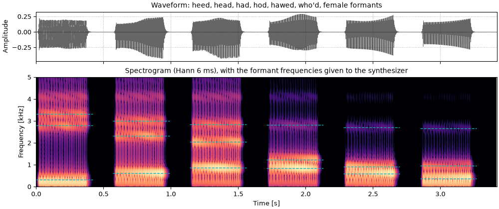
Peterson and Barney's female averages, for the same six vowels. Every formant is higher
than the male ones, since female vocal tracts are on average shorter, but not by one common
factor: the printout gives the ratios, from 1.04 to 1.30. The pitch is higher too, falling
from 230 to 200 Hz, and F4 and F5 are raised to 4100 and 4900 Hz to stay above the female F3.
Code
VOWELS_FEMALE = {
    "heed": (310, 2790, 3310),
    "head": (610, 2330, 2990),
    "had": (860, 2050, 2850),
    "hod": (850, 1220, 2810),
    "hawed": (590, 920, 2710),
    "who'd": (370, 950, 2670),
}
parts_female = []
for f1, f2, f3 in VOWELS_FEMALE.values():
    v = so.klatt_synthesize(
        VOWEL_DUR,
        FS,
        F0=([0, VOWEL_DUR], [230, 200]),
        AV=onoff(VOWEL_DUR),
        F1=f1,
        F2=f2,
        F3=f3,
        F4=4100,
        F5=4900,
    )
    parts_female += [v, gap]
for word, (f1, f2, f3) in VOWELS_FEMALE.items():
    male = VOWELS[word]
    ratios = ", ".join(f"{f / m:.2f}" for f, m in zip((f1, f2, f3), male, strict=True))
    print(f"{word:6} female / male, F1 F2 F3: {ratios}")
heed   female / male, F1 F2 F3: 1.15, 1.22, 1.10
head   female / male, F1 F2 F3: 1.15, 1.27, 1.21
had    female / male, F1 F2 F3: 1.30, 1.19, 1.18
hod    female / male, F1 F2 F3: 1.16, 1.12, 1.15
hawed  female / male, F1 F2 F3: 1.04, 1.10, 1.12
who'd  female / male, F1 F2 F3: 1.23, 1.09, 1.19
Six vowels with female formants
The six vowels with female formants. The harmonics are now about 215 Hz apart, so each
formant peak is drawn by fewer of them than in the male vowels above.
sound = finish(so.concat(parts_female))
tracks = [
    (np.repeat(starts, 2) + np.tile([0, VOWEL_DUR], 6), np.repeat([v[i] for v in VOWELS_FEMALE.values()], 2))
    for i in range(3)
]
fig, playhead = show(sound, "heed, head, had, hod, hawed, who'd, female formants")
for tt, ff in tracks:
    for j in range(6):
        playhead[1].plot(tt[2 * j : 2 * j + 2], ff[2 * j : 2 * j + 2] / 1000, color="c", lw=1, ls="--")
Male and female vowels by their first two formants
Both sets of vowels by their first two formants, joined vowel by vowel. The female vowel
space is shifted up and outward, most of all in F2 for the front vowels.
Code
fig, ax = plt.subplots(figsize=(5, 4), layout="constrained")
for word in VOWELS:
    (f1_male, f2_male, _), (f1_female, f2_female, _) = VOWELS[word], VOWELS_FEMALE[word]
    ax.plot([f2_male, f2_female], [f1_male, f1_female], color="0.7", lw=0.8)
    ax.annotate(word, (f2_female, f1_female), textcoords="offset points", xytext=(6, 4))
ax.plot([v[1] for v in VOWELS.values()], [v[0] for v in VOWELS.values()], "o", color="C0", label="male")
ax.plot(
    [v[1] for v in VOWELS_FEMALE.values()],
    [v[0] for v in VOWELS_FEMALE.values()],
    "o",
    color="C1",
    label="female",
)
ax.set(xlabel="F2 (Hz)", ylabel="F1 (Hz)", xlim=(3000, 600), ylim=(950, 200))
ax.legend(loc="lower left", fontsize=8)
ax.set_title("Peterson and Barney's averages, male and female")
Consonants from transitions
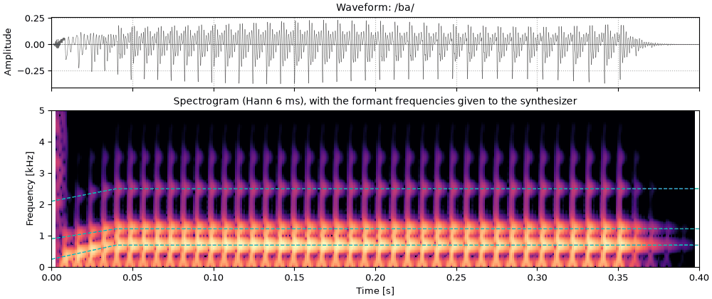
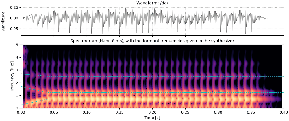
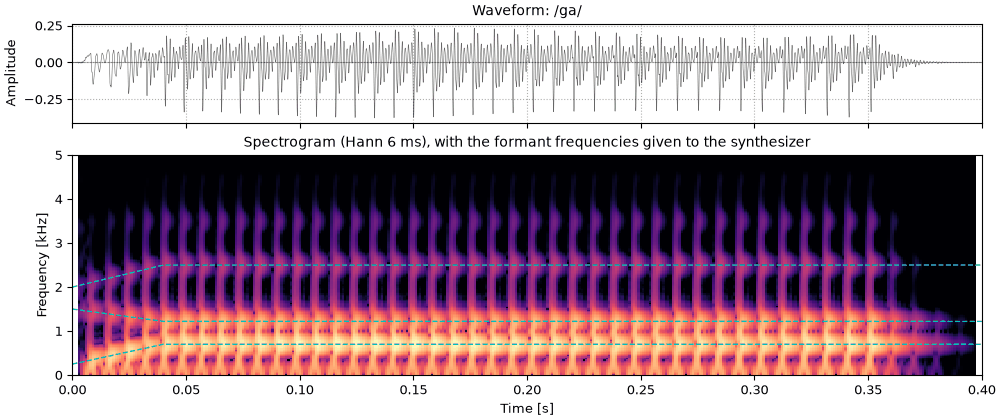
A stop consonant before a vowel is mostly heard in the first few tens of milliseconds of the
vowel: the formants move from where the closure left them to the vowel's values. Here F1 rises
from 250 Hz in each, and only the starting points of F2 and F3 differ. A short burst of
frication marks the release: flat for /b/, high for /d/, near F2 for /g/.
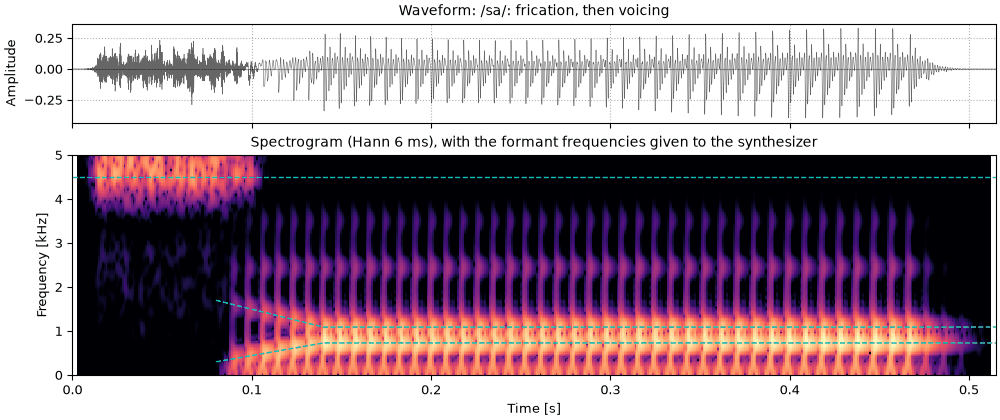
Klatt's synthesizer has two noise sources. Aspiration goes through the same formants as
voicing (the cascade), as the breath noise of /h/ does. Frication goes through a separate,
parallel set of formants, each with its own level, because a fricative's noise is made in a
constriction near the front of the mouth and excites mainly the resonances in front of it.
While voicing is on, both noises are modulated at F_0, 50% deep, as breath through vibrating
vocal folds is.
The syllable sa
/sa/: frication through the parallel formants 5 and 6 (4500 and 5500 Hz), then the vowel. As
in speech, there is no silence between them: the voicing starts while the frication is still
fading, and the first two formants glide from where the tongue left them (F1 low, F2 near
1700 Hz) to the vowel's values over the first 60 ms of voicing.
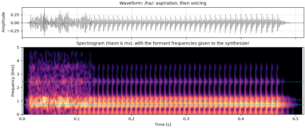
/ha/: aspiration alone through the vowel's formants, then voicing. The formants of the vowel
are already there in the breath, and the breath carries on into the first 50 ms or so of the
voicing, fading as it goes, so the vowel starts breathy.
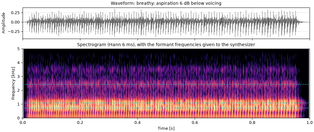
A breathy "hod": voicing with aspiration 6 dB below it throughout, and a wider first formant.
The noise fills in between the harmonics, most at high frequencies where the harmonics are
weak.
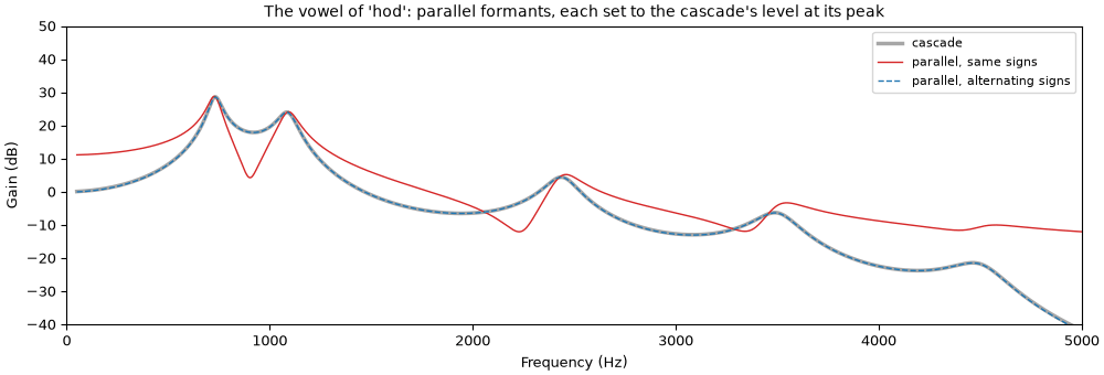
In the cascade, formants run one after another and their levels follow from their
frequencies. In the parallel branch each formant gets the source separately and is added at a
level of its own. Added with the same sign, neighbouring formants partly cancel between their
peaks, because their phases differ by about half a cycle there. Klatt adds them with
alternating signs, and then the sum follows the cascade closely, given the right levels.
Five formants in cascade, and in parallel with each sign rule
Code
f = np.linspace(50, 5000, 4000)
z = np.exp(-2j * np.pi * f / FS)


def response(fk, bk):
    c, b = -np.exp(-2 * np.pi * bk / FS), 2 * np.exp(-np.pi * bk / FS) * np.cos(2 * np.pi * fk / FS)
    return (1 - b - c) / (1 - b * z - c * z**2)


hs = [response(fk, bk) for fk, bk in HOD]
cascade = np.prod(hs, axis=0)
peaks = [np.argmin(np.abs(f - fk)) for fk, _ in HOD]
levels = [np.abs(cascade[i]) / np.abs(h[i]) for h, i in zip(hs, peaks, strict=True)]
same = sum(g * h for g, h in zip(levels, hs, strict=True))
alternating = sum((-1) ** k * g * h for k, (g, h) in enumerate(zip(levels, hs, strict=True)))

fig, ax = plt.subplots(figsize=(10, 3.4), layout="constrained")
db = lambda h: 20 * np.log10(np.abs(h))  # noqa: E731
ax.plot(f, db(cascade), color="k", lw=2.5, alpha=0.35, label="cascade")
ax.plot(f, db(same), color="C3", lw=1, label="parallel, same signs")
ax.plot(f, db(alternating), color="C0", lw=1, ls="--", label="parallel, alternating signs")
ax.set(xlabel="Frequency (Hz)", ylabel="Gain (dB)", xlim=(0, 5000), ylim=(-40, 50))
ax.set_title("The vowel of 'hod': parallel formants, each set to the cascade's level at its peak")
ax.legend(loc="upper right", fontsize=8)
Code
inside = (f > 100) & (f < 4000)
print("Largest difference from the cascade, 100-4000 Hz:")
print(f"  same signs        {np.abs(db(same) - db(cascade))[inside].max():5.1f} dB")
print(f"  alternating signs {np.abs(db(alternating) - db(cascade))[inside].max():5.1f} dB")
Largest difference from the cascade, 100-4000 Hz:
  same signs         13.7 dB
  alternating signs   0.1 dB
Voice quality
Everything above used Klatt's 1980 source, whose spectrum is fixed. The glottal pulse itself
changes with how the vocal folds are held: pressed together they close abruptly, which makes
strong high harmonics; held loosely they close gradually, leaving little but the fundamental.
The Liljencrants-Fant (LF) model (Fant, Liljencrants & Lin, 1985) describes one period of the
glottal flow's derivative E(t): an exponentially growing sinusoid while the glottis opens,
E(t) = E_0\, e^{\alpha t} \sin(\pi t / t_p), \qquad 0 \le t \le t_e,
down to its sharp negative peak -E_e at closure t_e, then an exponential return to zero.
Fant (1995) set the whole shape with one number,
R_d = \frac{U_0}{0.11\, E_e T_0},
the peak flow U_0 against the strength of the closure, in a period T_0: about 0.3 for a
tense, pressed voice to 2.7 for a lax, breathy one, and close to 0.7 for typical male
voices. so.glottal_source makes LF pulses from their harmonics, which have an exact
formula, so nothing aliases, and so.klatt_synthesize uses them with SS=3 (the source
switch of Klatt & Klatt's KLSYN88) and RD.
One period of the LF pulse at three values of Rd
The same peak excitation E_e in all three. The tense pulse opens for a shorter part of the
period and passes less air; the lax one stays open longer, and its closure is a gentle slope
rather than a sharp corner. The sharp corner is what makes high harmonics.
Code
x = np.linspace(0, 1, 1000)
RDS = {0.5: "tense, Rd 0.5", 1.0: "modal, Rd 1", 2.5: "lax, Rd 2.5"}
fig, (ax0, ax1) = plt.subplots(1, 2, figsize=(10, 3.2), layout="constrained")
for (rd, label), color in zip(RDS.items(), ["C3", "k", "C0"], strict=True):
    ax0.plot(x, so.lf_pulse(x, rd, flow=True), color=color, label=label)
    ax1.plot(x, so.lf_pulse(x, rd), color=color, label=label)
ax0.set(xlabel="Time (fraction of a period)", ylabel="Flow (units of $E_e T_0$)")
ax0.set_title("Glottal flow")
ax1.set(xlabel="Time (fraction of a period)", ylabel="$E(t)$ (units of $E_e$)")
ax1.set_title("Its derivative: the excitation, with radiation from the lips")
ax0.legend(fontsize=8)
The spectra of the three pulses, and of the 1980 source
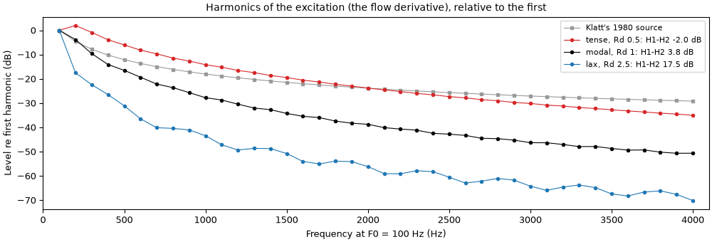
The harmonics' levels depend on the harmonic number only, not on F_0. The difference
between the first two harmonics, H1-H2, is the usual measure of this in recordings; Fant's
(1995) fit to it, -7.6 + 11.1\,R_d dB, agrees with these spectra to within 0.4 dB up to
R_d 1.4. Klatt's 1980 source has the H1-H2 of a modal voice, but around 3 kHz its harmonics
are stronger than even the tense pulse's.
Code
k = np.arange(1, 41)
klatt_1980 = gain(0, 100, k * 100) * np.abs(1 - np.exp(-2j * np.pi * k * 100 / FS))
fig, ax = plt.subplots(figsize=(10, 3.4), layout="constrained")
ax.plot(
    k * 100,
    20 * np.log10(klatt_1980 / klatt_1980[0]),
    "s-",
    ms=3,
    lw=0.8,
    color="0.6",
    label="Klatt's 1980 source",
)
for (rd, label), color in zip(RDS.items(), ["C3", "k", "C0"], strict=True):
    levels = 20 * np.log10(np.abs(so.lf_harmonics(k, rd)))
    levels -= levels[0]
    ax.plot(k * 100, levels, "o-", ms=3, lw=0.8, color=color, label=f"{label}: H1-H2 {-levels[1]:.1f} dB")
ax.set(xlabel="Frequency at F0 = 100 Hz (Hz)", ylabel="Level re first harmonic (dB)", xlim=(0, 4100))
ax.set_title("Harmonics of the excitation (the flow derivative), relative to the first")
ax.legend(fontsize=8)
One vowel, three voices
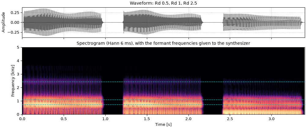
The vowel of "hod" three times, with everything the same except the pulse: tense (Rd 0.5),
modal (Rd 1) and lax (Rd 2.5). The vowel stays the same; the voice goes from pressed and
bright to soft and muffled.
fq3_one_vowel_three_voices.flac, 3.4 s, mono
Code
parts = []
for rd in RDS:
    snd = so.klatt_synthesize(DUR, FS, F0=F0, AV=onoff(DUR), SS=3, RD=rd, **hod)
    parts += [snd, so.silence(0.2, FS)]
sound = finish(so.concat(parts[:-1]))
fig, playhead = show(sound, "Rd 0.5, Rd 1, Rd 2.5", [730, 1090, 2440])
The 1980 source, then LF at Rd 0.7
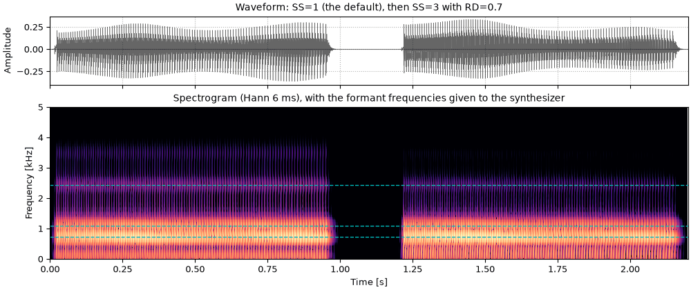
Klatt's 1980 source, then an LF pulse at the default Rd of 0.7, close to typical male voices.
The LF voice is darker: at 3 kHz its harmonics are about 12 dB weaker, relative to the first.
parts = [
    so.klatt_synthesize(DUR, FS, F0=F0, AV=onoff(DUR), **hod),
    so.silence(0.2, FS),
    so.klatt_synthesize(DUR, FS, F0=F0, AV=onoff(DUR), SS=3, **hod),
]
sound = finish(so.concat(parts))
fig, playhead = show(sound, "SS=1 (the default), then SS=3 with RD=0.7", [730, 1090, 2440])
Relaxing into breathy voice
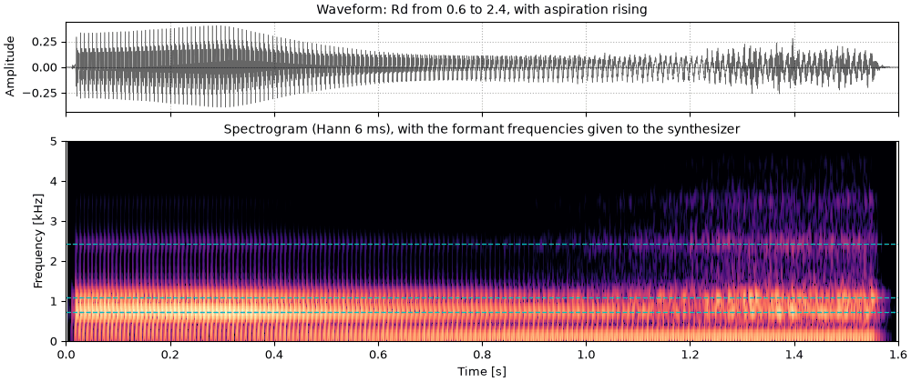
A voice relaxing at the end of a phrase: Rd rises from 0.6 to 2.4 while the pitch falls. The
LF model is the periodic pulse only, and a lax pulse alone sounds soft rather than breathy;
Klatt & Klatt (1990) found aspiration noise the most important cue to breathiness, so the
aspiration (AH) rises with Rd.
The rest of voice quality. KLSYN88 (Klatt & Klatt, 1990) has more voice controls than the LF pulse: open quotient, a spectral tilt filter, flutter (slow random jitter of F_0) and double pulsing, and its own polynomial pulse (KLGLOTT88). sonore has the LF pulse only.
Copying a recording. The parameters here were written by hand. Copy synthesis fits formant tracks to a recording, which needs a formant tracker that sonore does not have; the Voices from harmonics page rebuilds a recording from its measured pitch and envelope instead.
Rules. Text-to-speech systems drive formant synthesizers from phonetic rules, which generate the tracks from a transcription. Here every track is set by hand.
Drawing the tracks. Every track here is written in code. sonore-sketch, a separate browser app built on sonore, draws formant, F_0, voicing and bandwidth tracks with a mouse and plays what the synthesizer makes of them.
Fant (1995). The LF-model revisited. Transformations and frequency domain analysis. STL-QPSR 36(2–3), 119–156. The Rd parameter. waveforms.glottal_source
Fant, Liljencrants & Lin (1985). A four-parameter model of glottal flow. STL-QPSR 26(4), 1–13. waveforms.lf_harmonics
Klatt & Klatt (1990). Analysis, synthesis, and perception of voice quality variations among female and male talkers. J. Acoust. Soc. Am. 87(2), 820–857. doi:10.1121/1.398894. The SS source switch.
Peterson & Barney (1952). Control methods used in a study of the vowels. J. Acoust. Soc. Am. 24(2), 175–184. ASA. The vowels' formant frequencies.