Seeing speech

Motivation

A spectrogram is not only something to look at. Most of what speech analysis and synthesis measure is measured from a time-frequency representation, and whatever the representation smears, the measurement inherits. A few examples, all in this sentence:

• Pitch. An F0 estimator finds the spacing of the harmonics or the interval between glottal pulses, so it needs one or the other resolved. Its errors grow with harmonic number: if F_0 is off by \delta, the k-th harmonic is off by k\delta. At this speaker's typical F_0 of about 120 Hz, a 2% error moves the 20th harmonic, near 2.4 kHz, by 48 Hz, 0.4 of the gap to its neighbor. A vocoder that splits the voice into harmonics and noise on that grid counts the misplaced harmonic energy as noise, and resynthesizes it as such. An octave error, the most common failure, gets the pitch itself wrong by a factor of two.
• Spectral envelope. The formants are the envelope of the harmonics, and a vocoder needs that envelope without the excitation in it. A long window leaves a ripple at the harmonics; a short one flickers as pulses enter and leave it. Both come from the vocal folds, not the vocal tract, yet a synthesizer would reproduce them as if they were part of the voice's timbre. This is why vocoders such as STRAIGHT and WORLD tie the window to the pitch period.
• Glottal pulses. Pitch-synchronous processing, such as changing pitch or duration by moving whole periods, and voice-quality measures such as jitter, the cycle-to-cycle change in period, need the instant each pulse arrives. Only short windows, or reassignment, show it sharply.
• Change. The pitch of this sentence spans more than an octave, from below 90 Hz to above 190 Hz, and the formants sweep at every boundary between consonant and vowel. A fixed window long enough to resolve the harmonics at the bottom of that range smears them wherever the pitch moves.

No single fixed window serves all of these at once. The rest of the page shows why, and what each analysis in sonore does about it.

The sentence, and code the examples share

Every example below is the code shown with it, run after this cell: the sentence and its pitch track, the level the gallery plays sounds at, and the plotting conventions all images share.

import matplotlib
import matplotlib.pyplot as plt
import numpy as np
from matplotlib.collections import PatchCollection
from matplotlib.patches import Rectangle

import sonore as so

plt.rcParams.update({"font.size": 9, "axes.titlesize": 10, "figure.dpi": 100})


def finish(snd):
    """How every sound in the gallery is played: 5 ms ramps, RMS 0.1, peak at most 0.95."""
    snd = snd.ramp(5e-3).normalize(rms=0.1)
    return snd.normalize(peak=0.95) if snd.peak > 0.95 else snd


# The sentence at its native 16 kHz, and its F0 track (WORLD Harvest, 0 where unvoiced).
# Sources: docs/speech/SOURCES.md.
sentence = finish(so.load("docs/speech/bdl_arctic_a0131.flac"))
f0_times, f0 = np.loadtxt("docs/speech/bdl_arctic_a0131_f0.csv", delimiter=",", skiprows=2).T
fs = sentence.fs

# Every image on the page: dB re its own maximum over 60 dB, on a linear 0 to 5 kHz axis.
FMAX, DB = 5000, 60


def panels(n, height_ratios=None, height=7.4):
    fig = plt.figure(figsize=(10, height), layout="constrained")
    return fig, fig.subplots(n, 1, sharex=True, height_ratios=height_ratios)


def image(ax, rep, title, **kwargs):
    rep.plot(ax, db_range=DB, colorbar=False, fmax=FMAX, **kwargs)
    ax.set_title(title)


def shared_time(fig, axes, images):
    """The sentence's time axis on every panel, one colorbar for the images.
    Returns the panels, for the playhead to follow."""
    for ax in np.ravel(axes):
        ax.set_xlim(0, sentence.duration)
        ax.set_xlabel("")
    for ax in np.atleast_1d(axes[-1]):  # the bottom row
        ax.set_xlabel("Time [s]")
    sm = matplotlib.cm.ScalarMappable(matplotlib.colors.Normalize(-DB, 0), "magma")
    fig.colorbar(sm, ax=list(np.ravel(images)), label="dB re panel maximum", shrink=0.9)
    return list(np.ravel(axes))

One window, two views

The short-time Fourier transform (STFT) looks at the signal x through a window w slid to time t, and measures how much of each frequency f is in what it sees:

Each coefficient is the inner product of x with one atom, the window shifted to t and modulated to f. The atom has a duration, the window's, and a bandwidth, that of the window's spectrum W. Two sounds can be told apart in time only if they are further apart than the window is long, and in frequency only if they are further apart than W is wide.

Duration and bandwidth trade against each other. Measure each as a standard deviation, \sigma_t of the energy |w(\tau)|^2 over time and \sigma_f of |W(f)|^2 over frequency. Then for every window

with equality only for a Gaussian (Gabor, 1946). Stretching a window by a factor k multiplies \sigma_t by k and divides \sigma_f by k: the product, and the area of the atom's footprint in the time-frequency plane, stay the same.

The windows here are Hann windows, w(\tau) = \sin^2(\pi \tau / L) for 0 \le \tau \le L. A Hann window passes as much noise as an ideal bandpass filter of width 1.5/L, its equivalent noise bandwidth: 300 Hz for L = 5 ms, 45 Hz for L = 33.3 ms. Its product \sigma_t \sigma_f is within 3% of the bound, as the cell below measures on the windows sonore uses.

short = so.GaborFrame(0.002, 0.0005, n_fft=2048)  # Hann 2 ms, 0.5 ms hop
long = so.GaborFrame(0.1, 0.0005, n_fft=2048)  # Hann 100 ms
wide = so.GaborFrame(0.005, 0.001, n_fft=1024)  # Hann 5 ms, 1 ms hop
narrow = so.GaborFrame(0.0333, 0.001, n_fft=1024)  # Hann 33.3 ms


def spread(w, fs):
    """Standard deviations [s, Hz] of a window's energy in time, |w|², and in frequency, |W|²."""
    t = np.arange(len(w)) / fs
    p = w**2 / np.sum(w**2)
    sd_t = np.sqrt(np.sum(p * t**2) - np.sum(p * t) ** 2)
    W2 = np.abs(np.fft.fft(w, 256 * len(w))) ** 2  # finely interpolated spectrum
    f = np.fft.fftfreq(len(W2), 1 / fs)
    return sd_t, np.sqrt(np.sum(W2 * f**2) / np.sum(W2))


for frame in (short, wide, narrow, long):
    w = frame.window_samples(fs)
    sd_t, sd_f = spread(w, fs)
    enbw = fs * np.sum(w**2) / np.sum(w) ** 2
    print(
        f"Hann {1e3 * frame.win_dur:5.1f} ms: σt = {1e3 * sd_t:6.3f} ms, σf = {sd_f:6.1f} Hz, "
        f"σt·σf = {sd_t * sd_f:.4f}, noise bandwidth {enbw:5.0f} Hz"
    )
print(f"The bound 1/(4π) = {1 / (4 * np.pi):.4f}")

Hann   2.0 ms: σt =  0.283 ms, σf =  288.7 Hz, σt·σf = 0.0817, noise bandwidth   750 Hz
Hann   5.0 ms: σt =  0.707 ms, σf =  115.5 Hz, σt·σf = 0.0817, noise bandwidth   300 Hz
Hann  33.3 ms: σt =  4.712 ms, σf =   17.3 Hz, σt·σf = 0.0817, noise bandwidth    45 Hz
Hann 100.0 ms: σt = 14.145 ms, σf =    5.8 Hz, σt·σf = 0.0817, noise bandwidth    15 Hz
The bound 1/(4π) = 0.0796

Short and long windows

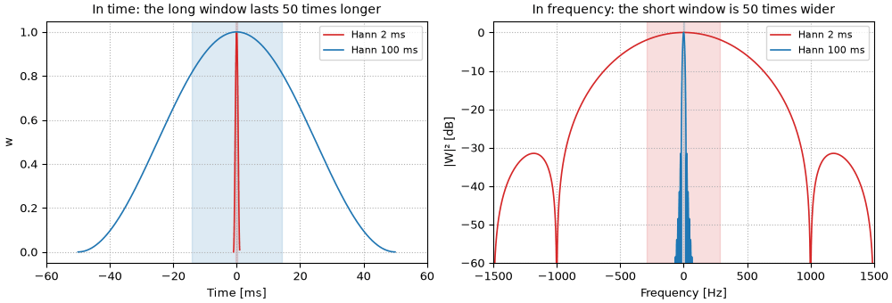
Two Hann windows fifty times apart in length, drawn to exaggerate the tradeoff: 2 ms and 100 ms. Left, the windows in time; right, their power spectra. The short window is over in a flash and smears every frequency across about 750 Hz; the long one lasts a tenth of a second and is only 15 Hz wide. The shaded bands are \pm\sigma_t and \pm\sigma_f.

Code

fig, (ax_t, ax_f) = plt.subplots(1, 2, figsize=(10, 3.4), layout="constrained")
for frame, color in ((short, "tab:red"), (long, "tab:blue")):
    w = frame.window_samples(fs)
    sd_t, sd_f = spread(w, fs)
    t = (np.arange(len(w)) - len(w) / 2) / fs
    label = f"Hann {1e3 * frame.win_dur:.0f} ms"
    ax_t.plot(1e3 * t, w, color=color, lw=1.2, label=label)
    ax_t.axvspan(-1e3 * sd_t, 1e3 * sd_t, color=color, alpha=0.15)
    W2 = np.abs(np.fft.fftshift(np.fft.fft(w, 2**17))) ** 2
    f = np.fft.fftshift(np.fft.fftfreq(2**17, 1 / fs))
    ax_f.plot(f, 10 * np.log10(np.maximum(W2 / W2.max(), 1e-12)), color=color, lw=1.2, label=label)
    ax_f.axvspan(-sd_f, sd_f, color=color, alpha=0.15)
ax_t.set(
    xlim=(-60, 60), xlabel="Time [ms]", ylabel="w", title="In time: the long window lasts 50 times longer"
)
ax_f.set(
    xlim=(-1500, 1500),
    ylim=(-60, 3),
    xlabel="Frequency [Hz]",
    ylabel="|W|² [dB]",
    title="In frequency: the short window is 50 times wider",
)
for ax in (ax_t, ax_f):
    ax.legend(loc="upper right", fontsize=8)
    ax.grid(ls=":")

Too short and too long

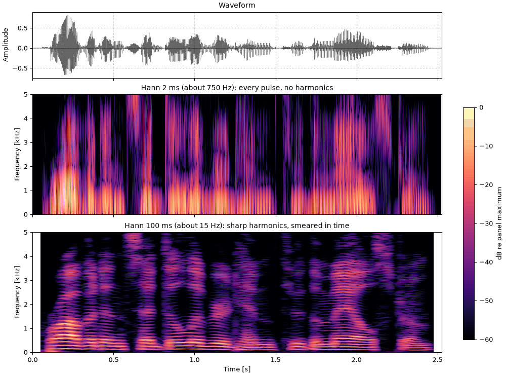
The same two windows on the sentence. Through 2 ms, shorter than one glottal period, each pulse of the voice is its own vertical line, sharp in time, but the harmonics are gone and even the formants blur into broad smudges. Through 100 ms, longer than a syllable's steady stretch, the harmonics are thin lines wherever the pitch holds still, but they smear wherever it moves, and onsets and stops spread over a tenth of a second.

w2_too_short_and_too_long.flac, 2.5 s, mono

Code

fig, axes = panels(3, [0.55, 1, 1])
sentence.plot(axes[0], color="k", lw=0.4)
axes[0].set_title("Waveform")
image(axes[1], short.analyze(sentence), "Hann 2 ms (about 750 Hz): every pulse, no harmonics")
image(axes[2], long.analyze(sentence), "Hann 100 ms (about 15 Hz): sharp harmonics, smeared in time")
playhead = shared_time(fig, axes, images=axes[1:])
sound = sentence

Wideband and narrowband

Speech is made of two things at two time scales. The vocal folds snap shut once per period, T_0 = 1/F_0, about 8 ms for this speaker (median F_0 121 Hz), and each pulse excites the vocal tract, whose resonances, the formants, shape the spectrum. The periodic pulses put energy at the harmonics kF_0; the formants decide which harmonics are loud.

A window much shorter than T_0 sees the pulses one at a time; a window longer than a few periods has a bandwidth narrower than F_0 and resolves the harmonics. Phoneticians settled on one of each, between the extremes above.

Two classic spectrograms

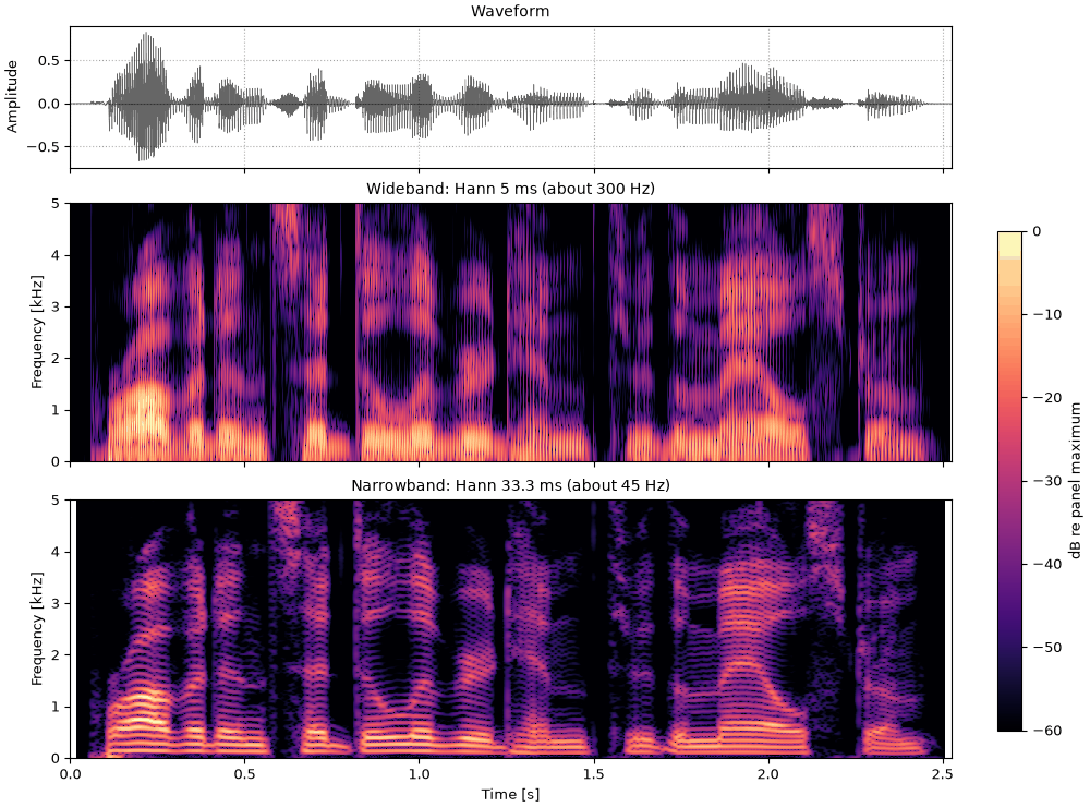
Hann windows with a 1 ms hop. The 5 ms window, about 300 Hz wide, makes a wideband spectrogram: each glottal pulse is a vertical striation and the formants are broad bands. The 33.3 ms window, about 45 Hz wide, makes a narrowband one: the harmonics are horizontal lines and the pulses are smeared out. Neither shows both.

27_two_classic_spectrograms.flac, 2.5 s, mono

Code

fig, axes = panels(3, [0.55, 1, 1])
sentence.plot(axes[0], color="k", lw=0.4)
axes[0].set_title("Waveform")
image(axes[1], wide.analyze(sentence), "Wideband: Hann 5 ms (about 300 Hz)")
image(axes[2], narrow.analyze(sentence), "Narrowband: Hann 33.3 ms (about 45 Hz)")
playhead = shared_time(fig, axes, images=axes[1:])
sound = sentence

Letting the window scale with frequency

Harmonics are evenly spaced, F_0 apart, but what matters to a listener is their spacing relative to their frequency: the 2nd and 3rd harmonics are far apart in this sense, the 30th and 31st nearly the same. A constant-Q analysis makes each filter's bandwidth proportional to its center frequency f_c, so its duration is inversely proportional: long windows for low frequencies, which resolve the first few harmonics, and short ones for high frequencies, which catch each pulse.

A Morlet wavelet with c cycles is a Gaussian in frequency whose width grows with f_c:

minus a small correction that makes it zero at 0 Hz. In time it is a tone at f_c under a Gaussian envelope of standard deviation c / (2\pi f_c): always about c cycles long, 6 here.

The cochlea is roughly constant-Q too, but its filters are causal: they cannot respond before the sound arrives. A gammatone filter, a standard model of one place on the basilar membrane, has the impulse response

with b = 1.019\,\mathrm{ERB}(f_c) and \mathrm{ERB}(f) = 24.7\,(4.37 f / 1000 + 1) Hz, the equivalent rectangular bandwidth of the human auditory filter (Glasberg & Moore, 1990). Its envelope peaks at t = 3 / (2\pi b) after a click, later for lower, narrower filters.

morlet = so.morlet_filterbank(54, 70, 7000, cycles=6)  # 54 wavelets, 70 Hz to 7 kHz, zero-phase
gammatone = so.gammatone_filterbank(60, 70, 7000)  # 60 filters, 2 per ERB, causal
latency = gammatone.envelope_peak_delay[1:-1]  # without the two edge filters
print(
    f"envelope-peak latency: {1e3 * latency[0]:.1f} ms at {gammatone.cfs[1]:.0f} Hz, "
    f"{1e3 * latency[-1]:.2f} ms at {gammatone.cfs[-2]:.0f} Hz"
)

envelope-peak latency: 14.5 ms at 70 Hz, 0.60 ms at 7000 Hz

Constant-Q and the cochlea

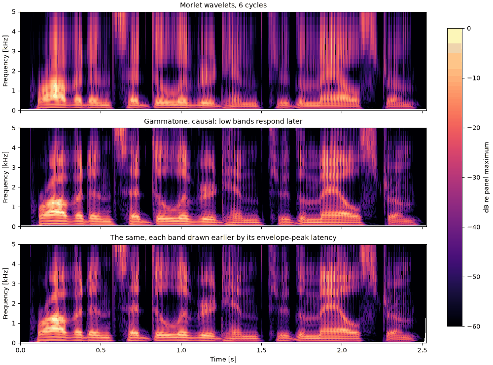
Here the bandwidth grows with frequency, so the low bands resolve single harmonics while the high bands are short enough to show each pulse. Top: 54 Morlet wavelets of 6 cycles, zero-phase. Middle: 60 causal gammatone filters, 2 per ERB. Its low bands respond later: their envelopes peak up to 15 ms after the high bands', so each pulse is drawn as a sweep. Bottom: the same envelopes, each band drawn earlier by its envelope-peak latency. Only the drawing moves; the data are unchanged.

28_constant-q_and_the_cochlea.flac, 2.5 s, mono

Code

fig, axes = panels(3)
kw = {"db_range": DB, "colorbar": False, "fscale": "linear", "fmax": FMAX}
morlet.analyze(sentence).envelopes(fs=1000).plot(axes[0], **kw)
axes[0].set_title("Morlet wavelets, 6 cycles")
env = gammatone.analyze(sentence).envelopes(fs=1000)
env.plot(axes[1], **kw)
axes[1].set_title("Gammatone, causal: low bands respond later")
env.plot(axes[2], align="peak", **kw)
axes[2].set_title("The same, each band drawn earlier by its envelope-peak latency")
playhead = shared_time(fig, axes, images=axes)
sound = sentence

Following the pitch

The voice's own time scale is its period, and that changes as the pitch moves. A window that is always 3 periods long,

has a noise bandwidth of 1.5 / L = F_0 / 2, so neighboring harmonics, F_0 apart, are always two bandwidths apart: they separate equally well at every pitch, with the shortest window that does so. sonore's time-varying Gabor frame steps these windows along with a hop of L/4. Through unvoiced stretches F_0 is bridged log-linearly between its voiced neighbors, so the window length never jumps.

Any window a few periods long still flickers: the power it collects rises and falls as pulses enter and leave it, with period T_0. TANDEM-STRAIGHT (Kawahara et al., 2011) cancels the flicker by averaging two spectrograms half a period apart, where its fundamental is in opposite phase:

with Blackman windows 2.5 periods long. The result is a power spectrum only: an average of two frames' magnitudes has no synthesis.

# t_end runs half a longest window past the end, so the last sample is covered evenly.
adaptive = so.TVGaborFrame.pitch_adaptive(f0_times, f0, t_end=sentence.duration + 0.02, periods=3)
lengths = 1e3 * np.asarray(adaptive.win_durs)
print(f"{len(lengths)} windows, {lengths.min():.1f} to {lengths.max():.1f} ms long")

417 windows, 15.6 to 34.2 ms long

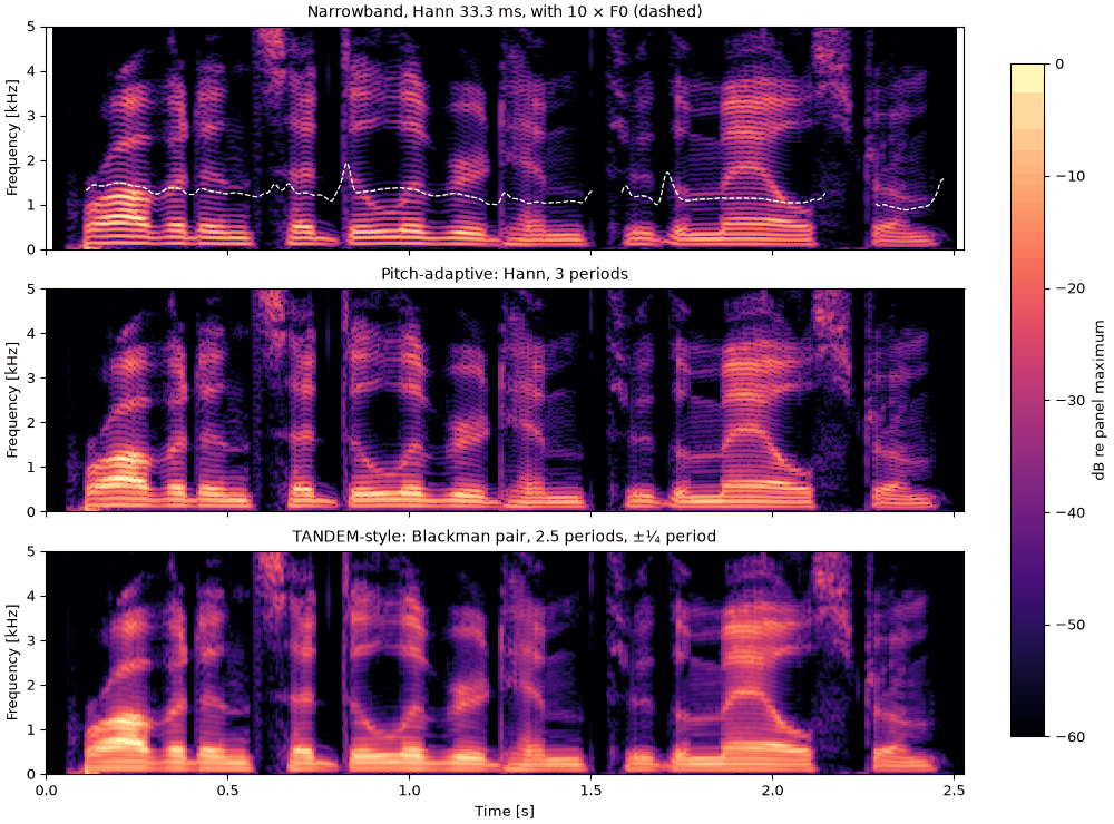
Following the pitch

Top: the narrowband spectrogram with ten times the F0 track (WORLD Harvest, where voiced), which should lie on the tenth harmonic. Middle: the time-varying frame whose Hann windows are 3 pitch periods long, so neighboring harmonics are separated equally well at every F0. Bottom: the TANDEM-STRAIGHT-style power spectrum. It is a power spectrum only, not TANDEM-STRAIGHT: no smoothing, no aperiodicity, no synthesis.

29_following_the_pitch.flac, 2.5 s, mono

Code

fig, axes = panels(3)
image(axes[0], narrow.analyze(sentence), "Narrowband, Hann 33.3 ms, with 10 × F0 (dashed)")
voiced = np.where(f0 > 0, 10 * f0 / 1000, np.nan)
axes[0].plot(f0_times, voiced, color="w", ls="--", lw=0.9)
image(axes[1], adaptive.analyze(sentence), "Pitch-adaptive: Hann, 3 periods")
image(axes[2], so.tandem_power(sentence, f0_times, f0), "TANDEM-style: Blackman pair, 2.5 periods, ±¼ period")
playhead = shared_time(fig, axes, images=axes)
sound = sentence

The same plane, tiled four ways

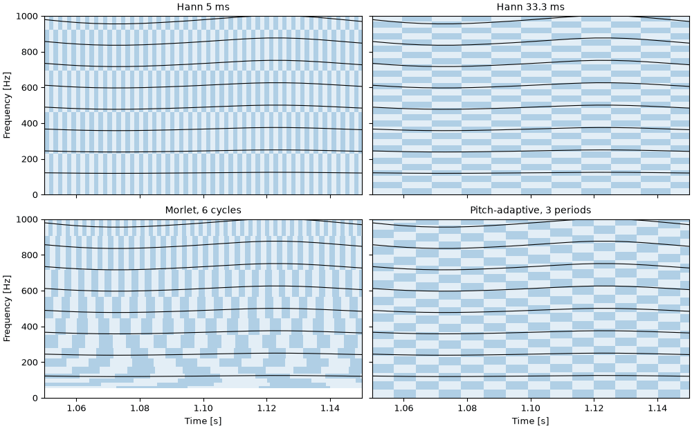
Each analysis divides the time-frequency plane into cells of about the same area, and differs only in their shape and in how the shape changes across the plane. The figure draws one box per cell, 2\sigma_t wide and 2\sigma_f tall, over a tenth of a second of the sentence, with the harmonics kF_0(t) drawn over them in black. A harmonic is resolved where the boxes are shorter than the gap between harmonics; a pulse is resolved where they are narrower than the period.

Four tilings

Fixed windows tile the plane with identical boxes: flat ones for 5 ms, tall ones for 33.3 ms. Morlet boxes are tall and narrow at high frequencies and wide and flat at low ones, so only the lowest harmonics are resolved. Pitch-adaptive boxes are always the same fraction of the harmonic spacing tall, about 0.4, and widen and narrow as the pitch falls and rises.

Code

t_lo, t_hi, f_hi = 1.05, 1.15, 1000
sd_t, sd_f = spread(long.window_samples(fs), fs)
hann_t, hann_f = sd_t / long.win_dur, sd_f * long.win_dur  # σt = 0.141 L and σf = 0.577 / L for any L
is_voiced = f0 > 0


def f0_at(t):  # bridged across unvoiced stretches, as the pitch-adaptive frame does
    return np.exp(np.interp(t, f0_times[is_voiced], np.log(f0[is_voiced])))


# Each box is (time, frequency, width, height, column, row); column + row picks its shade.
def grid(L):  # boxes of a fixed Hann window of length L
    dt, df = 2 * hann_t * L, 2 * hann_f / L
    times, freqs = np.arange(t_lo + dt / 2, t_hi + dt, dt), np.arange(df / 2, f_hi + df, df)
    return [(t, f, dt, df, i, j) for i, t in enumerate(times) for j, f in enumerate(freqs)]


def wavelet_boxes(c=6):  # sd c/(2π fc) of the amplitude envelope; energy sds are 1/√2 of those
    boxes, a, fc, j = [], 1 / (c * np.sqrt(2)), 60.0, 0
    while fc < f_hi + fc * a:
        dt, df = 2 * c / (2 * np.pi * fc * np.sqrt(2)), 2 * a * fc
        boxes += [(t, fc, dt, df, i, j) for i, t in enumerate(np.arange(t_lo + dt / 2, t_hi + dt, dt))]
        fc, j = fc * (1 + a) / (1 - a), j + 1  # the next box starts where this one ends
    return boxes


def pitch_boxes(periods=3):
    boxes, t, i = [], t_lo, 0
    while t < t_hi:
        L = periods / f0_at(t)
        dt, df = 2 * hann_t * L, 2 * hann_f / L
        boxes += [(t + dt / 2, f, dt, df, i, j) for j, f in enumerate(np.arange(df / 2, f_hi + df, df))]
        t, i = t + dt, i + 1
    return boxes


fig, axes = plt.subplots(2, 2, figsize=(10, 6.2), sharex=True, sharey=True, layout="constrained")
tilings = [
    (grid(0.005), "Hann 5 ms"),
    (grid(0.0333), "Hann 33.3 ms"),
    (wavelet_boxes(), "Morlet, 6 cycles"),
    (pitch_boxes(), "Pitch-adaptive, 3 periods"),
]
tt = np.linspace(t_lo, t_hi, 200)
for ax, (boxes, title) in zip(axes.flat, tilings, strict=True):
    for k in range(1, int(f_hi / 90)):
        ax.plot(tt, k * f0_at(tt), color="k", lw=0.8)
    rects = [Rectangle((t - dt / 2, f - df / 2), dt, df) for t, f, dt, df, _, _ in boxes]
    shade = [0.35 if (i + j) % 2 else 0.12 for *_, i, j in boxes]  # a checkerboard
    ax.add_collection(PatchCollection(rects, facecolor=[(0.12, 0.47, 0.71, a) for a in shade], lw=0))
    ax.set(title=title, xlim=(t_lo, t_hi), ylim=(0, f_hi))
for ax in axes[1]:
    ax.set_xlabel("Time [s]")
for ax in axes[:, 0]:
    ax.set_ylabel("Frequency [Hz]")

Reassignment

A spectrogram cell reports energy at its own center (t, f), even when that energy comes from a pulse near the edge of the window or a harmonic between two bins. Reassignment moves each cell to the center of gravity of its energy (Kodera et al., 1978; Auger & Flandrin, 1995):

where X_w is the STFT with the window w, X_{\tau w} with the time-weighted window \tau w(\tau), and X_{w'} with its derivative. A pure tone lands on its frequency, an impulse on its time, and a linear chirp on its instantaneous frequency, whatever the window. The moved energy is then summed into display bins.

Reassignment

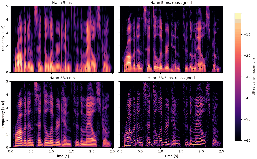
Left: the 5 ms and 33.3 ms spectrograms. Right: the same, with each cell's energy moved to its center of gravity in time and frequency, then summed into bins of about one pixel, 5 ms by 20 Hz (cells more than 60 dB below the maximum are dropped). Reassignment sharpens what the window already resolves, pulses with the short window and harmonics with the long one; it does not escape the choice of window. It is not a frame and has no synthesis.

30_reassignment.flac, 2.5 s, mono

Code

fig = plt.figure(figsize=(10, 6.2), layout="constrained")
axes = fig.subplots(2, 2, sharex=True, sharey=True)
# Bins of about one pixel of these panels (5 ms by 20 Hz): finer bins would be drawn by
# skipping cells, coarser ones would blur what reassignment sharpened.
t_edges = np.arange(0, sentence.duration + 5e-3, 5e-3)
f_edges = np.arange(0, FMAX + 20, 20)
for row, (frame, name) in enumerate(((wide, "5 ms"), (narrow, "33.3 ms"))):
    image(axes[row, 0], frame.analyze(sentence), f"Hann {name}")
    rs = so.reassigned_spectrogram(sentence, frame).binned(t_edges, f_edges)
    image(axes[row, 1], rs, f"Hann {name}, reassigned")
    axes[row, 1].set_ylabel("")
playhead = shared_time(fig, axes, images=axes)
sound = sentence

A higher voice

Everything above used one male voice. Female voices sit about half an octave to an octave higher, and that changes which picture works. Here is the same sentence read by a female talker (CMU ARCTIC, speaker slt). The female harmonics are about one and a half times as far apart as the male ones, so:

• The narrowband window resolves the female harmonics even more clearly, since they are further apart than its bandwidth by a wider margin.
• The wideband window, 5 ms, is now nearly one female period long, so it no longer sees one pulse at a time and the female striations blur.
• Each formant is drawn by fewer harmonics, so the envelope between harmonics is a guess. This is why female voices have long been harder to analyze: at an F_0 of 200 Hz and above, a formant peak that falls between two harmonics is simply not in the spectrum. docs/design/views/female-voices.md measures how much the envelope estimates suffer.

The pitch-adaptive window adjusts by itself: three female periods are about 16 ms. The F0 track here is from so.f0_track, sonore's own tracker, since this recording has no stored track.

# The same sentence read by a female talker, and its F0 track from sonore's tracker.
sentence_female = finish(so.load("docs/speech/slt_arctic_a0131.flac"))
track_female = so.f0_track(sentence_female)
f0_female = track_female.f0[0]
voiced_female = f0_female[f0_female > 0]
print(f"median F0: {np.median(f0[f0 > 0]):.0f} Hz (bdl), {np.median(voiced_female):.0f} Hz (slt)")
adaptive_female = so.TVGaborFrame.pitch_adaptive(
    track_female.t, f0_female, t_end=sentence_female.duration + 0.02, periods=3
)
lengths_female = 1e3 * np.asarray(adaptive_female.win_durs)
print(f"pitch-adaptive windows for slt: {lengths_female.min():.1f} to {lengths_female.max():.1f} ms long")

median F0: 121 Hz (bdl), 183 Hz (slt)
pitch-adaptive windows for slt: 13.3 to 20.1 ms long

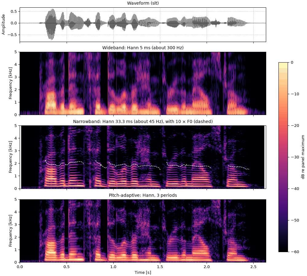
The same sentence, a higher voice

The female talker's sentence through the windows used above for the male talker's. Top: the waveform. Then the wideband spectrogram, Hann 5 ms, where the female pulses, about 5.5 ms apart, are barely separate. Then the narrowband one, Hann 33.3 ms, with ten times the female F0 (dashed), where the female harmonics stand well apart. Bottom: the pitch-adaptive frame, 3 female periods long. Compare with Two classic spectrograms and Following the pitch.

f1_the_same_sentence_a_higher_voice.flac, 2.6 s, mono

Code

fig, axes = panels(4, [0.55, 1, 1, 1], height=9.0)
sentence_female.plot(axes[0], color="k", lw=0.4)
axes[0].set_title("Waveform (slt)")
image(axes[1], wide.analyze(sentence_female), "Wideband: Hann 5 ms (about 300 Hz)")
image(
    axes[2], narrow.analyze(sentence_female), "Narrowband: Hann 33.3 ms (about 45 Hz), with 10 × F0 (dashed)"
)
axes[2].plot(
    track_female.t, np.where(f0_female > 0, 10 * f0_female / 1000, np.nan), color="w", ls="--", lw=0.9
)
image(axes[3], adaptive_female.analyze(sentence_female), "Pitch-adaptive: Hann, 3 periods")
playhead = shared_time(fig, axes, images=axes[1:])
for ax in axes:
    ax.set_xlim(0, sentence_female.duration)
sound = sentence_female

Nothing is lost

Every analysis above except the last two is a frame: its coefficients determine the signal, and sonore's synthesize recovers it. For the STFT with window w and hop H, overlap-adding the windowed inverse transforms gives back the signal multiplied by

with K the FFT length, so synthesis divides by s(t), which works wherever the windows leave no gap. A filterbank's analogue is s(f) = \sum_k |H_k(f)|^2, divided out in frequency. The cell below resynthesizes the sentence from each frame's coefficients.

frames = {
    "Hann 2 ms": short,
    "Hann 5 ms": wide,
    "Hann 33.3 ms": narrow,
    "Hann 100 ms": long,
    "Morlet": morlet,
    "gammatone": gammatone,
    "pitch-adaptive": adaptive,
}
for name, frame in frames.items():
    back = frame.synthesize(frame.analyze(sentence))
    error = np.max(np.abs(back.data - sentence.data)) / sentence.peak
    print(f"{name:>15}: largest error {error:.1e} of the peak")

      Hann 2 ms: largest error 2.7e-16 of the peak
      Hann 5 ms: largest error 2.7e-16 of the peak
   Hann 33.3 ms: largest error 4.0e-16 of the peak
    Hann 100 ms: largest error 1.2e-15 of the peak
         Morlet: largest error 4.7e-16 of the peak
      gammatone: largest error 1.5e-15 of the peak
 pitch-adaptive: largest error 5.4e-16 of the peak

Every frame returns the sentence to within floating-point rounding. So the time-frequency tradeoff is not a loss of information: it appears only once the phase is discarded and the magnitudes are drawn. Which magnitude shows speech best depends on what you look for: pulses, harmonics, formants, or the pitch itself.

References

• Auger & Flandrin (1995). Improving the readability of time-frequency and time-scale representations by the reassignment method. IEEE Trans. Signal Processing 43(5). doi:10.1109/78.382394. spectra.reassigned_spectrogram
• Gabor (1946). Theory of communication. Part 1: The analysis of information. J. IEE 93(26). doi:10.1049/ji-3-2.1946.0074. gabor.GaborFrame
• Glasberg & Moore (1990). Derivation of auditory filter shapes from notched-noise data. Hearing Research 47. doi:10.1016/0378-5955(90)90170-T. filterbank.Gammatone
• Kawahara et al. (2011). Technical foundations of TANDEM-STRAIGHT, a speech analysis, modification and synthesis framework. Sādhanā 36(5). doi:10.1007/s12046-011-0043-3. spectra.tandem_power
• Kodera, Gendrin & de Villedary (1978). Analysis of time-varying signals with small BT values. IEEE Trans. ASSP 26(1). doi:10.1109/TASSP.1978.1163047. spectra.reassigned_spectrogram
• Kominek & Black (2004). The CMU Arctic speech databases. Proc. 5th ISCA Speech Synthesis Workshop, 223–224. ISCA Archive. The sentence, by speakers bdl and slt.