A modulation spectrum is the two-dimensional Fourier transform of a sound's envelopes, band by
band over time: how much of the pattern moves at each rate (Hz, across) and at each density
(cycles per octave, up), keeping only the magnitude (Singh & Theunissen, 2003). The
ripples page goes from a pattern to its spectrum. This page goes the other way:
from a spectrum, measured and edited or drawn from scratch, to a sound that has it.
A magnitude is not enough to make a sound. The spectrum has dropped the phase of the
modulations, which says when each event happens, and the fine structure under each band's
envelope. ModulationSpectrum.to_sound(carrier=...) takes both from a carrier, the way an
envelope is put back on a carrier: a sound lends its own, while "tones" and "noise" draw a
random modulation phase and put the envelopes on steady tones or on noise.
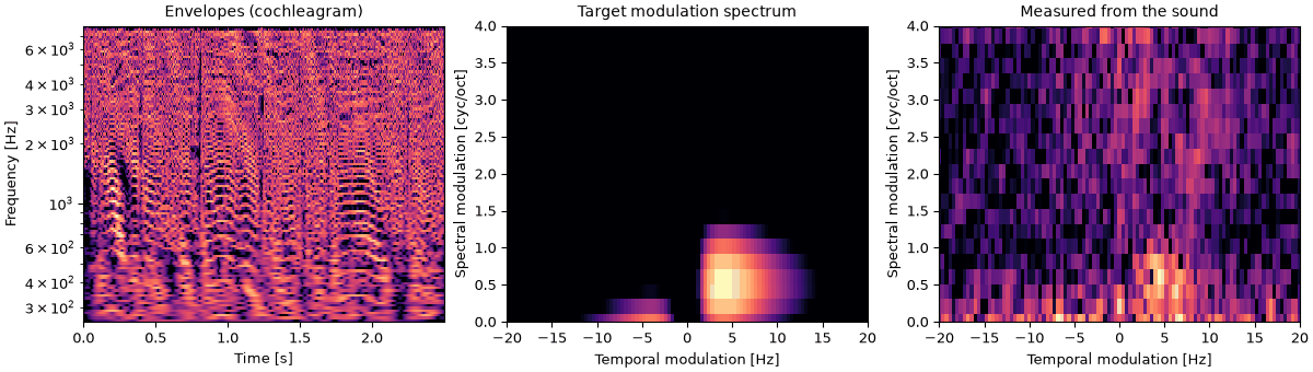
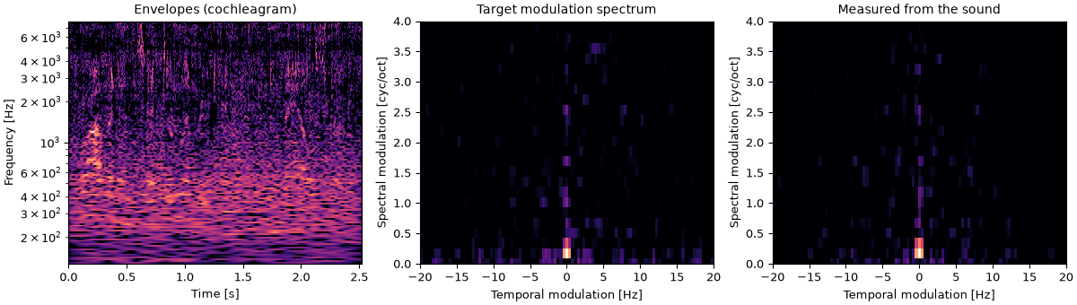
Same spectrum, different sound: a sentence and a sound with the sentence's modulation spectrum and random modulation phase.
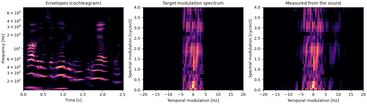
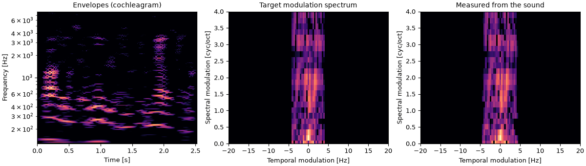
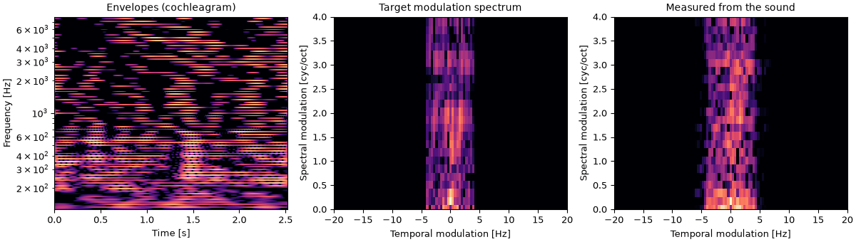
A drawn spectrum: one patch of modulation, heard on three carriers.
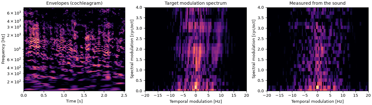
An edited sentence: a sentence with every modulation faster than 4 Hz removed, and how close the sound comes to that.
import matplotlib.pyplot as plt
import numpy as np

import sonore as so

plt.rcParams.update({"font.size": 9, "axes.titlesize": 10, "figure.dpi": 100})
FS = 44100


def finish(snd):
    """How every sound in the gallery is played: 5 ms ramps, RMS 0.1, peak at most 0.95."""
    snd = snd.ramp(5e-3).normalize(rms=0.1)
    return snd.normalize(peak=0.95) if snd.peak > 0.95 else snd


def measure(snd, f_lo):
    """The modulation spectrum on the page's grid: 12 bands per octave from f_lo to 8 kHz."""
    return so.ModulationSpectrum.octave(snd, f_lo=f_lo, f_hi=8000)


def show(snd, target=None, f_lo=250):
    """The sound's envelopes (a cochleagram), the target spectrum if there is one, and the
    spectrum measured from the sound. Returns the figure and the panel the playhead follows."""
    n_panels = 2 if target is None else 3
    fig, axes = plt.subplots(1, n_panels, figsize=(4 * n_panels, 3.4), layout="constrained")
    bank = so.cosine_filterbank(f_lo=f_lo, f_hi=8000, spacing=1 / 24, scale="octave")
    bank.analyze(snd).envelopes(lowpass=200, fs=1000).plot(axes[0], db_range=30, colorbar=False)
    axes[0].set_title("Envelopes (cochleagram)")
    if target is not None:
        target.plot(axes[1], db_range=30, wt_max=20, wf_max=4, colorbar=False)
        axes[1].set_title("Target modulation spectrum")
    measure(snd, f_lo).plot(axes[-1], db_range=30, wt_max=20, wf_max=4, colorbar=False)
    axes[-1].set_title("Measured from the sound")
    return fig, [axes[0]]
Press play and a line follows the sound across every time axis in its plots. Click any time
axis to play from that point. Start with your volume low.
Same spectrum, different sound
A sentence's modulation spectrum, measured in 12 bands per octave from 125 Hz to 8 kHz, then
heard with the sentence's own modulation phase thrown away. to_sound with carrier="tones"
draws a random phase, builds the envelopes from it and the stored magnitudes, and puts each one
on a steady tone at its band's centre. The random phase leaves the zero-rate column alone,
since that column (its phase as well as its magnitudes) is the sentence's long-term spectrum:
which bands are loud.
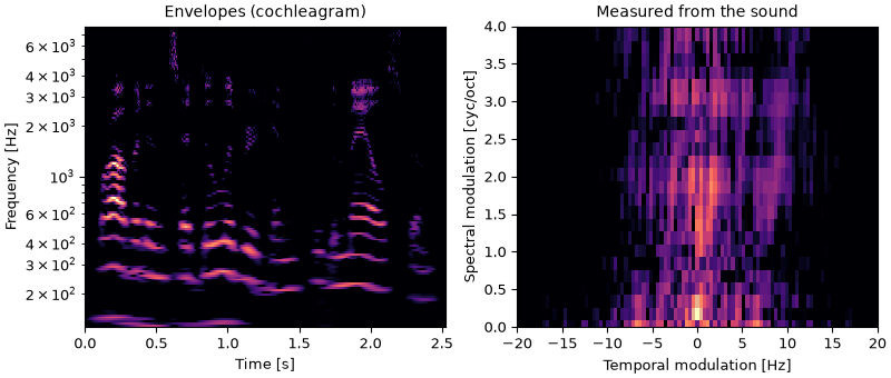
A sentence
The sentence, a male talker reading one of the CMU ARCTIC prompts. Its modulation spectrum
is brightest at low rates and densities, as for most natural sounds (Singh & Theunissen,
2003).
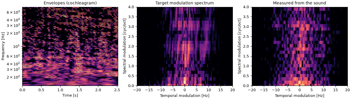
The same magnitudes with a random modulation phase. The syllables, the pauses and the onsets
are gone from the envelopes, which change at the sentence's rates and densities but never at
its moments. A random phase also asks for envelopes below zero, which no
envelope can be: about a third of the values (34% here) are clipped at zero, with a warning,
and that is why the measured spectrum is smoother than the target. The colour is kept only
roughly. A two-dimensional modulation spectrum does not say which bands carry which
modulation, so the random phase spreads the sentence's modulation into bands that were quiet,
and clipping turns it into level there.
So a modulation spectrum fixes how a sound changes, not when. In the design note's check of
the same sentence (docs/design/views/modulation-targets.md, C1) the two envelope arrays
correlate at −0.08, and the pooled envelope, more than 30 dB below its peak 9.6% of the time
in the sentence, never is in the twin. Sounds made this way, with a natural sound's modulation
spectrum and a random modulation phase, have been used to ask what auditory neurons respond
to (Hsu et al., 2004).
A drawn spectrum
A target can be drawn from scratch as a few patches on the rate × density plane.
so.ModulationBlob(rate, density) is a Gaussian bump at that rate [Hz] and density
[cycles/octave], half an octave wide in rate and a quarter of a cycle per octave in density by
default. The signs follow the ripples: a positive rate and density is a
downward sweep. A ripple is a blob of no width.
A drawing sets a shape, not a depth, so from_blobs takes the depth separately: rms_depth,
the rms of the envelopes about their mean, relative to the mean (0.2 by default). Envelopes
cannot go below zero, and a random phase reaches only a limited depth before they would: about
0.28 for the blob below (C2 of the design note), against 0.71 for one full ripple. A drawn
target that would need clipping is refused, with the largest depth that fits.
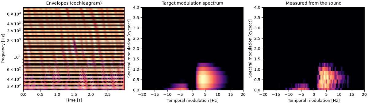
A drawn blob, on tones
Downward sweeps around 4 Hz and half a cycle per octave, on steady tones at the band centres.
Unlike a ripple, the sweeps come at irregular moments and with varying slopes, since the blob
spreads over a range of rates and densities and the phase is random. The faint patch at
negative rates along the bottom is the tail of the blob's mirror image at (−4 Hz, −0.5
cycle/octave), which every real pattern has.
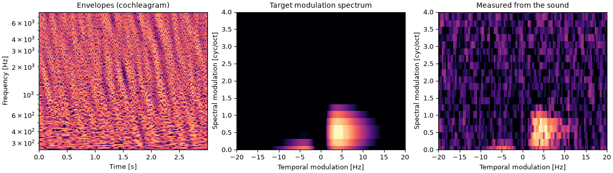
The same target on noise: each envelope multiplies a band of noise instead of a tone. The
sweeps are still there, under a hiss whose own random fluctuations fill the whole modulation
spectrum.
The same target on the sentence. A sound as carrier lends its own modulation phase as well as
its fine structure, so the sweeps now come when the sentence's syllables did, in its voice. The
sentence is 2.5 s long, so this target is drawn for 2.5 s.
How much of each sound's measured modulation power lies where the target has its power (within
20 dB of its peak), leaving out the zero-rate column, which holds the long-term spectrum:
Code
def share_in_target(snd, target):
    """Share of the measured modulation power, off the zero-rate column, inside the target."""
    measured = measure(snd, f_lo=250)
    measured_power = 10 ** (measured.level / 10)
    in_target = target.level > target.level.max() - 20
    moving = measured.w_t != 0
    return measured_power[in_target & moving].sum() / measured_power[:, moving].sum()


for name, snd, drawn in [
    ("tones", on_tones, target),
    ("noise", on_noise, target),
    ("sentence", on_sentence, short_target),
]:
    print(f"{name:>8}: {share_in_target(snd, drawn):.0%}")
   tones: 98%
   noise: 31%
sentence: 24%
The carrier matters as much as the target. A steady tone at each band's centre adds almost no
modulation of its own, so the target survives. Noise and speech fluctuate inside every band,
and those fluctuations land in the measured spectrum on top of the drawn one. That is why
"tones" is the default carrier (C3 of the design note).
An edited sentence
A measured spectrum can be edited and heard. with_gain(g) multiplies every cell by
g(rate, density); lambda r, d: abs(r) <= 4 keeps only the modulations at 4 Hz and below,
roughly the syllable rate and slower, and removes everything faster. Elliott & Theunissen
(2009) filtered the modulation spectrum of speech's spectrogram in a similar way to find which
modulations intelligibility needs. With the sentence itself as carrier, its own modulation phase and fine
structure go back under the edited magnitudes, so wherever the gain is 1 the timing is kept.
Modulations above 4 Hz removed
The edit, put straight back on the sentence. The measured spectrum keeps some power above
4 Hz, less than the sentence had but more than the edit asks for: the sentence's fine
structure brings fast modulation of its own back into every band.
The same edit with 20 rounds of a search in the manner of Griffin & Lim (1984): analyse the
sound, keep its fine structure and modulation phase, impose the edited magnitudes again, and
resynthesize. Each round brings the sound's own spectrum closer to the edit.
The modulation power left between 6 and 40 Hz, relative to the sentence's:
Code
def fast_share(snd):
    """Share of the measured modulation power at 6-40 Hz."""
    measured = measure(snd, f_lo=125)
    power = 10 ** (measured.level / 10)
    fast = (np.abs(measured.w_t) >= 6) & (np.abs(measured.w_t) <= 40)
    return power[:, fast].sum() / power.sum()


for name, snd in [("edit", edited), ("20 iterations", searched), ("on tones", on_tones_edit)]:
    print(f"{name:>13}: {10 * np.log10(fast_share(snd) / fast_share(sentence)):.1f} dB")
         edit: -4.1 dB
20 iterations: -16.3 dB
     on tones: -12.9 dB
None of them reaches the edit exactly, which removed everything there. A sound's envelopes are
not free: they come from filtering one waveform, so most arrays of magnitudes belong to no
sound at all, and the search finds a sound whose spectrum is close, never equal. The design
note measures the same comparison in C6 and C7.
Timing from one sound, magnitudes from another
A sound as carrier lends its modulation phase, so one sound's magnitudes can be heard with
another sound's timing. to_envelopes(carrier=...) gives the envelopes alone, which can then go
on either sound's fine structure. Here the sentence and 2.5 s of rain trade halves.
Code
rain = so.load("docs/textures/rain.flac").mono().resample(sentence.fs)
rain = so.Sound(rain.data[: sentence.n_samples], sentence.fs)
rain_spectrum = measure(rain, f_lo=125)
bank = spectrum._analysis.filterbank  # the 12-per-octave bank both spectra were measured with
Rain magnitudes, sentence timing
Rain's modulation magnitudes and fine structure, with the sentence's modulation phase. The
rain now swells and fades with the syllables.
The other way round: the sentence's magnitudes and fine structure, with rain's modulation
phase. The voice is still there, but its events come at rain's moments.
Some of the words can be made out in both: speech carries information in its timing and in
its modulation spectrum.
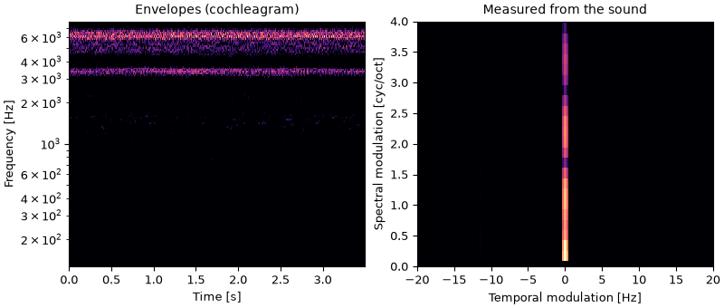
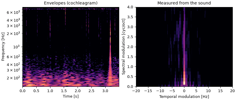
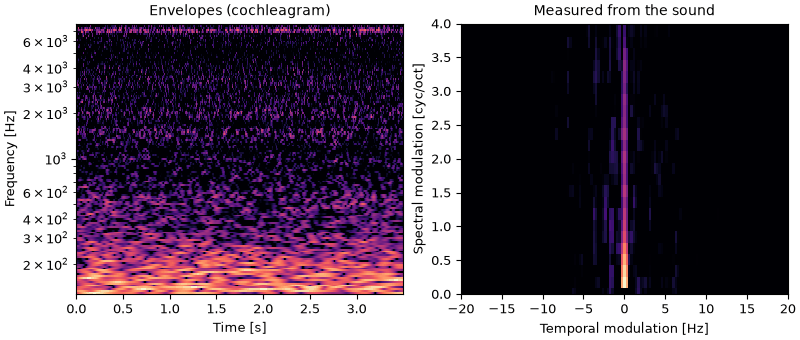
Twins band by band
A two-dimensional modulation spectrum says how much modulation there is at each rate and
density, but not which bands carry it. A random phase therefore spreads modulation into bands
that were steady or quiet, which is the extra noise heard in the sentence's twin above. A
narrower description keeps it: each band's own modulation spectrum, the per-band modulation
power that McDermott & Simoncelli (2011) use among their texture statistics. A twin of that
keeps each band's envelope magnitudes over rate and randomizes only its phase in time, band by
band. Both kinds of twin below keep each band's own fine structure, so only the envelopes
differ.
Code
def band_twin(snd, rng=0):
    """Each band keeps its envelope's magnitude spectrum over time (and so its level); the phase is
    random, band by band. On the sound's own fine structure."""
    bank = so.cosine_filterbank(f_lo=125, f_hi=8000, spacing=1 / 12, scale="octave")
    subbands = bank.analyze(snd)
    envelopes = subbands.envelopes(fs=1000).data[:, :, 0]  # (time, band)
    magnitude = np.abs(np.fft.rfft(envelopes, axis=0))
    phase = np.random.default_rng(rng).uniform(0, 2 * np.pi, magnitude.shape)
    phase[0] = 0  # each band's mean stays
    rebuilt = np.fft.irfft(magnitude * np.exp(1j * phase), n=len(envelopes), axis=0)
    twin_envelopes = so.Envelopes(np.maximum(rebuilt, 0), 1000, bank)
    return (twin_envelopes * subbands.tfs()).to_sound()


def plane_twin(snd, rng=0):
    """The same modulation spectrum on the plane, a random phase, on the sound's own fine structure."""
    plane = measure(snd, f_lo=125)
    subbands = plane._analysis.filterbank.analyze(snd)
    return (plane.to_envelopes(rng=rng) * subbands.tfs()).to_sound()


def texture(name, seconds=3.5):
    snd = so.load(f"docs/textures/{name}.flac").mono()
    return so.Sound(snd.data[: int(seconds * snd.fs)], snd.fs)
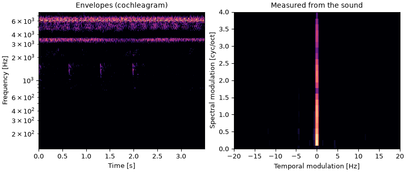
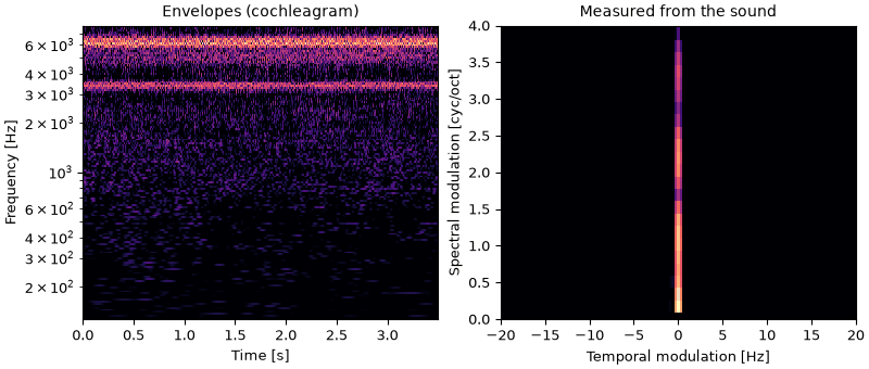
The crickets' twin on the plane. The long-term spectrum is kept, so the chirps stay at the
top, but some of their modulation spreads into the bands below, which were nearly silent.
The fire's twin band by band. Every band keeps its level and its modulation spectrum, but the
crackles are gone: a crackle is a brief event in many bands at once, and that alignment lives
in the phase.
So a band-by-band twin keeps a steady texture such as crickets, rain or wind, but not the
sparse events of a fire, applause or speech. That is why McDermott & Simoncelli's statistics
also include each band's envelope skew and kurtosis and the correlations between bands.
What this page leaves out
Drawing with a mouse. Targets here are written in code, as blobs or as edits. sonore-sketch, a separate browser app built on sonore, draws them with a mouse: blobs on the plane, or cuts on a sound's measured spectrum.
dB targets. A spectrum measured with scale="db" (of the log envelope, as Elliott & Theunissen, 2009, define it) also goes back to sound, and never needs clipping, but the linear spectrum of the result is not the one drawn.
The other modulation spectra. A modulation spectrogram changes over time and has no route back to sound, and a sound texture's per-band modulation power is set through its statistics, not here.