Binaural cues

A sound off to one side reaches the nearer ear sooner and louder: an interaural time difference (ITD) and an interaural level difference (ILD). How alike the two ears' signals are, their interaural correlation, decides whether the image is a compact point or a diffuse cloud. Each example on this page changes one of these and holds the others still. They need headphones: over speakers the two ears' signals mix in the room and the effects disappear.

For real sources at real positions, with every cue together, see Moving talkers, where three talkers are rendered through measured head-related impulse responses and one of them moves.

Press play and a line follows the sound across every time axis in its plots. Click any time axis to play from that point. The audio is lossless, since compression would alter the binaural sounds. Start with your volume low.

How the cues are measured

so.interaural_cues cuts the two ears' signals into short windows (10 ms here) and, in each, finds the ITD as the lag of the peak of the interaural cross-correlation, the ILD as the level ratio, and the correlation both at zero lag and at its peak over lags (the coherence). It can also do this per frequency band, given a filterbank; here it uses the whole signal. Each figure shows the waveforms, the ITD and ILD, and the two correlations, all measured from the sound you hear.

Code
import matplotlib.pyplot as plt

import sonore as so

plt.rcParams.update({"font.size": 9, "axes.titlesize": 10, "figure.dpi": 100})
FS = 44100


def finish(snd):
    """How every sound in the gallery is played: 5 ms ramps, RMS 0.1, peak at most 0.95."""
    snd = snd.ramp(5e-3).normalize(rms=0.1)
    return snd.normalize(peak=0.95) if snd.peak > 0.95 else snd


def show(snd):
    """Waveforms, ITD and ILD, and interaural correlation, all on one time axis.
    Returns the figure and the panels the playhead follows."""
    fig, axes = plt.subplots(3, 1, figsize=(10, 6.6), sharex=True, layout="constrained")
    snd.plot(axes[0], lw=0.4)
    axes[0].set_title("Waveform, left and right")
    cues = so.interaural_cues(snd, win_dur=10e-3)
    cues.plot(axes[1])
    axes[1].set_xlabel("")
    axes[2].plot(cues.t, cues.corr0, color="tab:orange", lw=1, label="correlation at zero lag")
    axes[2].plot(cues.t, cues.iac, color="k", alpha=0.6, lw=1, label="coherence (peak over lags)")
    axes[2].axhline(0, color="k", alpha=0.25, lw=0.8)
    axes[2].set(ylim=(-1.05, 1.05), ylabel="Interaural corr.", xlabel="Time [s]", xlim=(0, snd.duration))
    axes[2].legend(loc="lower right", fontsize=8)
    axes[2].grid(ls=":")
    return fig, list(axes)
Timing alone

Timing alone 🎧

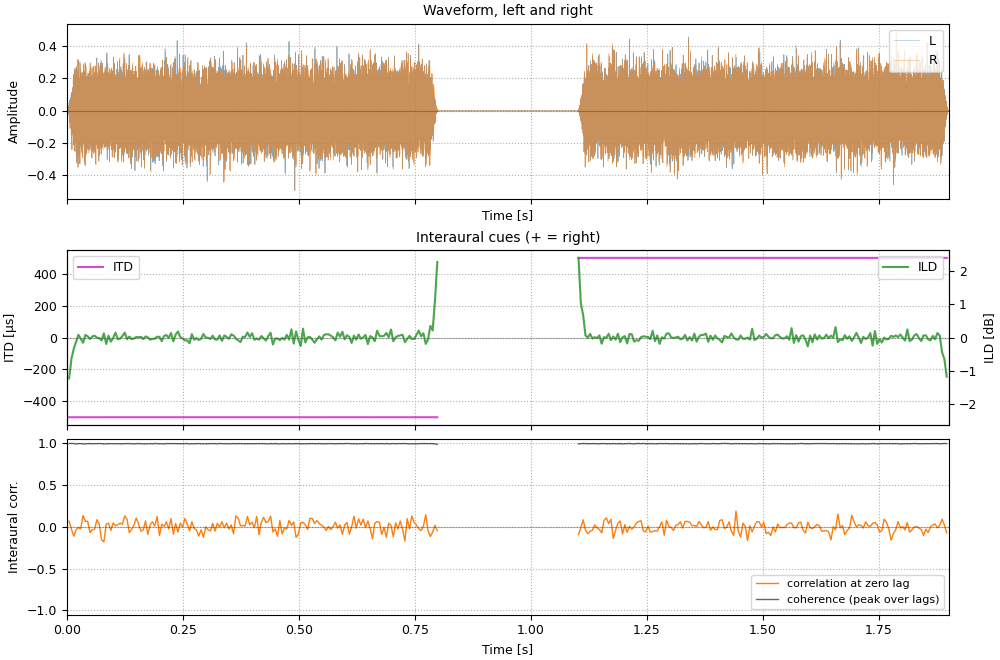
Noise with a 500 µs interaural time difference, leading in the left ear and then in the right. The level difference is zero throughout; the sideways shift comes from timing.

10_timing_alone.flac, 1.9 s, stereo

Plots of the timing alone sound
Code
noise = so.gaussian_noise(0.8, FS, rng=0).ramp(20e-3)
noise2 = so.gaussian_noise(0.8, FS, rng=1).ramp(20e-3)
sound = finish(
    so.concat(
        [
            so.apply_itd_ild(noise, itd=-500e-6),
            so.silence(0.3, FS),
            so.apply_itd_ild(noise2, itd=500e-6),
        ]
    )
)
fig, playhead = show(sound)

Correlation that changes

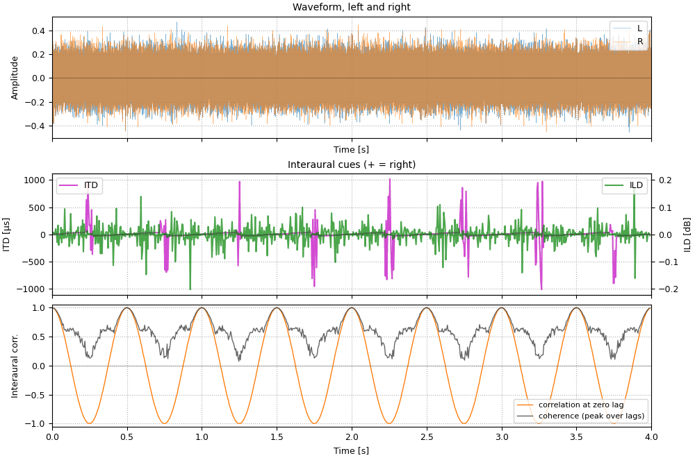
Siveke et al. (2008) made two noises whose interaural correlation changes over time while each ear alone hears plain noise, to ask how fast the binaural system can follow. In Oscor the right ear's noise is a moving mixture of the left ear's and an independent one; in phasewarp the right ear hears the left ear's noise shifted slightly in frequency, so every component's interaural phase rotates.

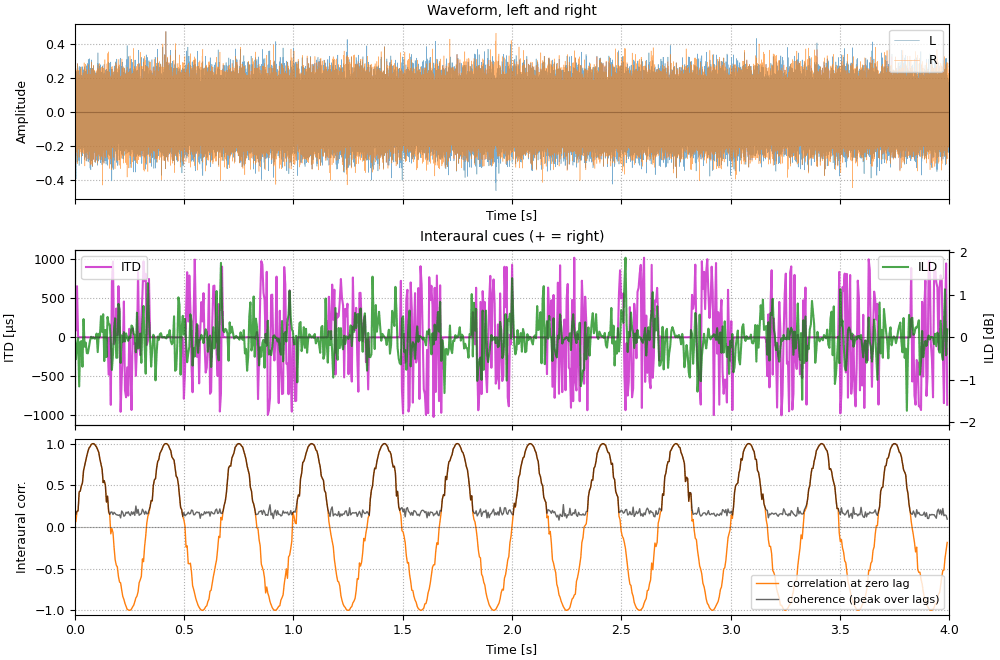
Oscor 🎧

Interaural correlation swings between +1 and −1 three times a second. The image in your head alternates between focused and diffuse; only the correlation panel shows what changes.

07_oscor.flac, 4.0 s, stereo

Plots of the oscor sound
Code
sound = finish(so.oscor(4, FS, f_mod=3, rng=0))
fig, playhead = show(sound)

Phasewarp 🎧

The interaural phase of every component rotates through 360° twice a second, so the zero-lag correlation follows a 2 Hz cosine.

08_phasewarp.flac, 4.0 s, stereo

Plots of the phasewarp sound
Code
sound = finish(so.phasewarp(4, FS, f_mod=2, rng=0))
fig, playhead = show(sound)

References