Iterated rippled noise

How it is made

so.iterated_ripple_noise starts from Gaussian noise x and repeats y \leftarrow y + g\,y(t - d) for the given number of iterations n (the "add-same" network; network="add-original" adds the delayed copy to the original noise instead). In frequency the delay-and-add is a comb filter, so the whole network is

whose peaks, with g = 1, sit at multiples of 1/d and grow sharper with each iteration. In time, the noise becomes partly correlated with itself d later: its autocorrelation has a peak at lag d, and its height, which grows with n, goes with how strong the pitch is. sonore computes the network exactly in the frequency domain, so the delay need not be a whole number of samples, and drops a warm-up stretch so that the noise is stationary from the start.

import matplotlib.pyplot as plt
import numpy as np

import sonore as so

plt.rcParams.update({"font.size": 9, "axes.titlesize": 10, "figure.dpi": 100})
FS = 44100


def finish(snd):
    """How every sound in the gallery is played: 5 ms ramps, RMS 0.1, peak at most 0.95."""
    snd = snd.ramp(5e-3).normalize(rms=0.1)
    return snd.normalize(peak=0.95) if snd.peak > 0.95 else snd


def show(snd):
    """so.overview: waveform, spectrum, spectrogram (50 ms windows) and modulation spectrum.
    Returns the figure and the panels the playhead follows."""
    fig = so.overview(snd, win_dur=50e-3, figsize=(10, 6.2), fmax=4000)
    return fig, [ax for ax in fig.axes if ax.get_title() in ("Waveform", "Spectrogram")]

Pitch from delay

Iterated rippled noise

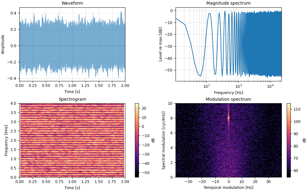
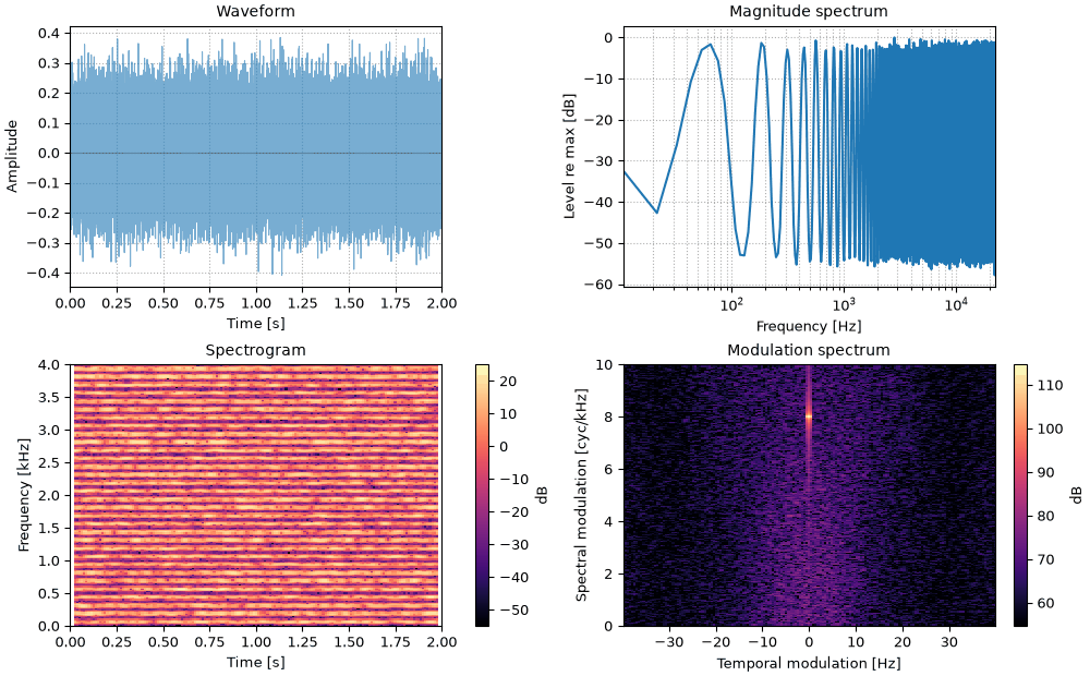
Noise added to an 8 ms delayed copy of itself, sixteen times over. A 125 Hz pitch rises out of the hiss; the spectrum ripples at multiples of 125 Hz and the modulation spectrum peaks at 8 cycles/kHz, the delay in milliseconds.

09_iterated_rippled_noise.flac, 2.0 s, mono

Code

sound = finish(so.iterated_ripple_noise(2, FS, delay=8e-3, iterations=16, rng=0))
fig, playhead = show(sound)

Fewer iterations

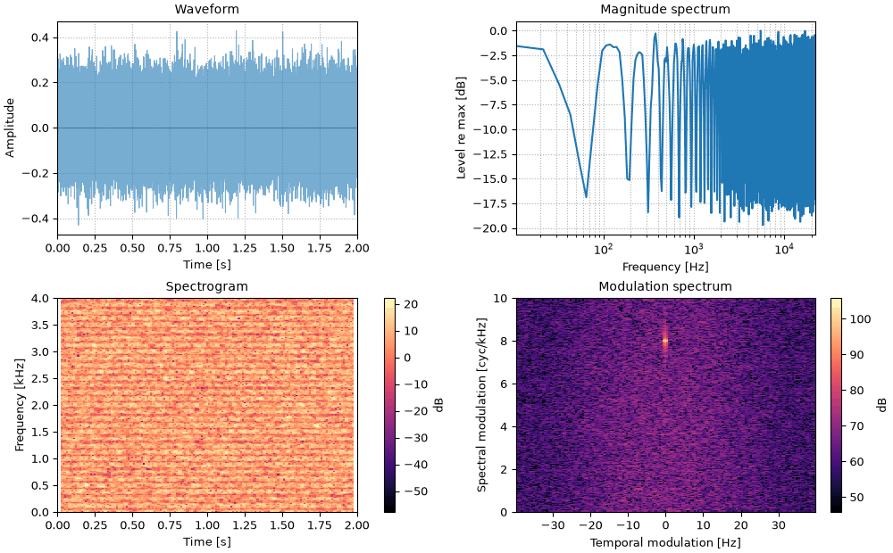
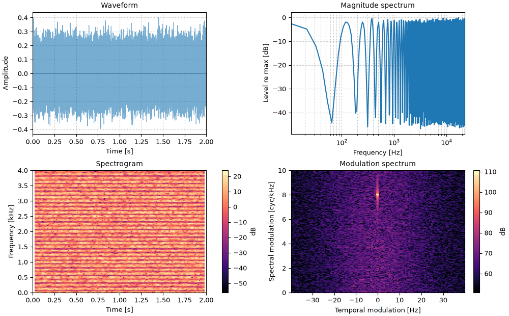
The same delay and the same noise, with fewer iterations. The ripple in the spectrum is shallower and the autocorrelation peak at 8 ms lower, and the pitch is weaker.

One iteration

One iteration: noise plus a single delayed copy. The spectrum is a gentle cosine ripple, and the pitch is faint, a coloring of the hiss rather than a note.

i1_one_iteration.flac, 2.0 s, mono

Code

sound = finish(so.iterated_ripple_noise(2, FS, delay=8e-3, iterations=1, rng=0))
fig, playhead = show(sound)

Four iterations

Four iterations: the peaks at multiples of 125 Hz are sharper, and the pitch is clear.

i4_four_iterations.flac, 2.0 s, mono

Code

sound = finish(so.iterated_ripple_noise(2, FS, delay=8e-3, iterations=4, rng=0))
fig, playhead = show(sound)

Autocorrelation and iterations

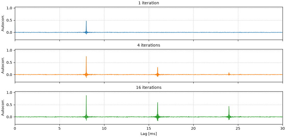
The normalized autocorrelation of each sound over its first 30 ms. The peak at 8 ms grows with the number of iterations (0.47, 0.75 and 0.88), and so do the peaks at its multiples.

Code

fig, axes = plt.subplots(3, 1, figsize=(10, 4.8), sharex=True, layout="constrained")
for ax, n, color in zip(axes, (1, 4, 16), ("tab:blue", "tab:orange", "tab:green"), strict=True):
    x = so.iterated_ripple_noise(2, FS, delay=8e-3, iterations=n, rng=0).data[:, 0]
    X = np.fft.rfft(x, 2 * len(x))
    r = np.fft.irfft(np.abs(X) ** 2)[: int(0.030 * FS)]
    ax.plot(1e3 * np.arange(len(r)) / FS, r / r[0], color=color, lw=1)
    ax.set(ylim=(-0.3, 1.05), ylabel="Autocorr.", title=f"{n} iteration{'s' * (n > 1)}")
    ax.grid(ls=":")
axes[-1].set(xlabel="Lag [ms]", xlim=(0, 30))

Subtracting instead

Negative gain

Sixteen iterations with gain g = -1: the delayed copy is subtracted. The spectral peaks move to odd multiples of 62.5 Hz, halfway between the ones above, and the autocorrelation at 8 ms turns negative, with the first positive peak at 16 ms. The pitch is ambiguous: neither simply 125 Hz nor an octave below (Yost, 1996).

in_negative_gain.flac, 2.0 s, mono

Code

sound = finish(so.iterated_ripple_noise(2, FS, delay=8e-3, gain=-1, iterations=16, rng=0))
fig, playhead = show(sound)

Rippled noise and moving ripples

The rippled spectrum here is one kind of ripple; the spectrotemporal ripples are another. This one does not move, so all of it sits at zero rate in a modulation spectrum, and it is periodic along linear frequency, one peak every 1/d hertz: an 8 ms delay gives 8 cycles/kHz, where the modulation spectrum of the first example peaks. Spectrotemporal ripples are sinusoidal along log frequency and drift over time. Equally spaced peaks along linear frequency are harmonics of 1/d, which is why rippled noise has a pitch and those ripples do not.

References

• Yost (1996). Pitch of iterated rippled noise. J. Acoust. Soc. Am. 100(1), 511–518. JASA (PDF). waveforms.iterated_ripple_noise