Analysis and resynthesis

Many of sonore's analyses can be run backwards: split a sound into bands or time-frequency cells, change what you find there, and synthesize a sound from the result. This page goes from doing nothing to removing the noise from a mixture.

Three other pages go further: the Phase vocoder changes a sound's duration, pitch or partials, Hearing through a vocoder keeps only band envelopes, and Cepstral analysis splits a voice into its vocal tract and its source.

Code
import matplotlib.pyplot as plt
import numpy as np

import sonore as so
from sonore import dB

plt.rcParams.update({"font.size": 9, "axes.titlesize": 10, "figure.dpi": 100})
FS = 44100


def finish(snd):
    """How every sound in the gallery is played: 5 ms ramps, RMS 0.1, peak at most 0.95."""
    snd = snd.ramp(5e-3).normalize(rms=0.1)
    return snd.normalize(peak=0.95) if snd.peak > 0.95 else snd

Press play and a line follows the sound across every time axis in its plots. Click any time axis to play from that point. Start with your volume low.

Perfect reconstruction

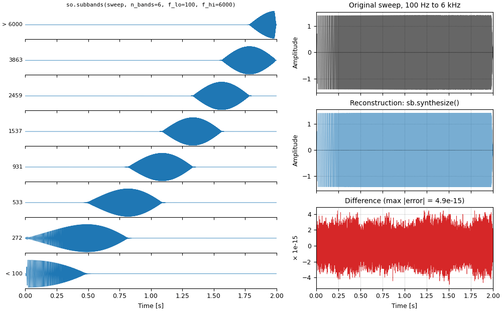
so.cosine_filterbank splits a sound with half-cosine filters equally spaced on the ERB scale, plus a lowpass and a highpass filter at the edges. Their squared responses sum to 1 at every frequency, so analysis followed by synthesis (each band filtered again, then summed) gives back the original, up to floating-point rounding.

Code
def show_bands(original):
    """The six bands of the sweep beside the original, the reconstruction and their difference.
    Returns the figure and the panels the playhead follows."""
    fig = plt.figure(figsize=(10, 6.2), layout="constrained")
    left, right = fig.subfigures(1, 2, width_ratios=[1.35, 1])
    sb = so.cosine_filterbank(6, 100, 6000).analyze(original)
    band_axes = left.subplots(len(sb), 1, sharex=True)
    sb.plot(band_axes)
    band_axes[0].set_title(
        "so.cosine_filterbank(6, 100, 6000).analyze(sweep)", family="monospace", fontsize=8
    )
    r = right.subplots(3, 1, sharex=True)
    original.plot(r[0], color="k", lw=0.4)
    r[0].set(title="Original sweep, 100 Hz to 6 kHz", xlabel="")
    recon = sb.to_sound()  # recomputed: the played sound has been level-normalized
    recon.plot(r[1], color="tab:blue", lw=0.4)
    r[1].set(title="Reconstruction: sb.to_sound()", xlabel="")
    err = recon - original
    r[2].plot(err.t, 1e15 * err.data[:, 0], color="tab:red", lw=0.5)
    r[2].set(title=f"Difference (max |error| = {err.peak:.1e})", ylabel="× 1e-15", xlabel="Time [s]")
    r[2].grid(ls=":")
    return fig, list(band_axes) + list(r)

Perfect reconstruction

An exponential sweep split into 6 ERB-spaced bands plus the lowpass and highpass edge filters, then summed back. What you hear is the reconstruction; it differs from the original only at the level of floating-point rounding.

26_perfect_reconstruction.flac, 2.0 s, mono

Plots of the perfect reconstruction sound
Code
sweep = so.exponential_chirp(2.0, FS, 100, 6000).ramp(20e-3)
sound = finish(so.cosine_filterbank(6, 100, 6000).analyze(sweep).to_sound())
fig, playhead = show_bands(sweep)

Masking the spectrogram

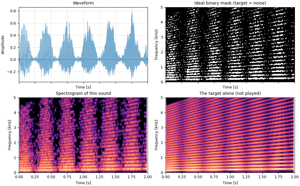
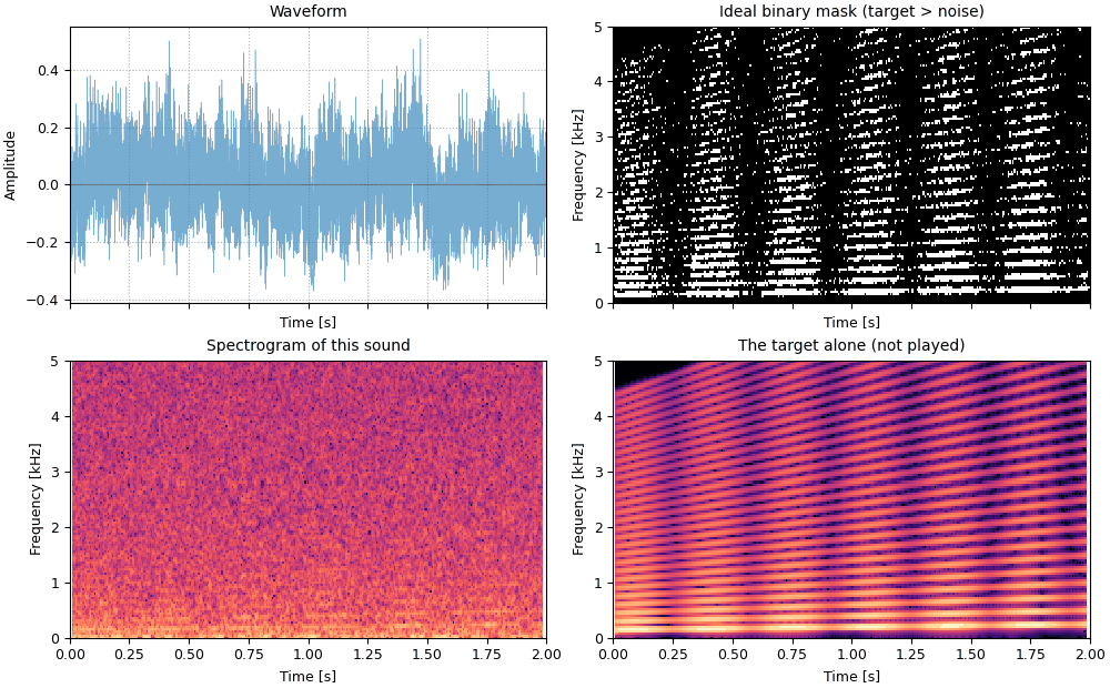
The STFT is invertible too, so a spectrogram with some of its cells switched off is still a sound. Wang (2005) proposed the ideal binary mask as the goal of separating speech from noise: keep every cell where the target is louder than the noise, discard the rest. It is ideal because computing it needs the target and the noise separately, which a listener never has; what a listener hears through it shows how much a perfect separation would leave.

Code
def gliding_target(dur=2.0):
    """A harmonic complex gliding 150 -> 250 Hz with a 3 Hz level fluctuation: a stand-in for speech."""
    t = np.arange(int(dur * FS)) / FS
    phase = 2 * np.pi * np.cumsum(150 + 50 * t) / FS
    target = so.Sound(sum(np.cos(k * phase) / k for k in range(1, 30)), FS).normalize()
    return (target * (0.6 + 0.4 * np.sin(2 * np.pi * 3 * t))).ramp(20e-3)


def show_mask(snd, target, mask):
    """Waveform, the mask, and spectrograms of this sound and of the target alone.
    Returns the figure and the panels the playhead follows."""
    fig, axes = plt.subplots(2, 2, figsize=(10, 6.2), sharex=True, layout="constrained")
    snd.plot(axes[0, 0], lw=0.4)
    axes[0, 0].set_title("Waveform")
    mask.plot(axes[0, 1])
    axes[0, 1].set(title="Ideal binary mask (target > noise)", ylim=(0, 5))
    so.STFT(snd, 25e-3).plot(axes[1, 0], fmax=5000, colorbar=False)
    axes[1, 0].set_title("Spectrogram of this sound")
    so.STFT(target, 25e-3).plot(axes[1, 1], fmax=5000, colorbar=False)
    axes[1, 1].set_title("The target alone (not played)")
    return fig, [axes[0, 0], axes[1, 0]]


target = gliding_target()
masker = so.gaussian_noise(target.duration, FS, tilt=-3, rng=0)
mixture = target + (masker + 5 * dB)
S_t, S_m, S_x = (so.STFT(x, 25e-3) for x in (target, masker, mixture))
mask = so.ideal_binary_mask(S_t, S_m, lc_db=0)
Target in noise

A gliding harmonic target (a stand-in for a voice) in pink noise at −5 dB SNR.

24_target_in_noise.flac, 2.0 s, mono

Plots of the target in noise sound
Code
sound = finish(mixture)
fig, playhead = show_mask(sound, target, mask)

Ideal binary mask

The same mixture with every time-frequency cell where the noise dominates switched off. The mask is computed from the separate target and noise, which is what makes it ideal; the resynthesis is exact.

25_ideal_binary_mask.flac, 2.0 s, mono

Plots of the ideal binary mask sound
Code
sound = finish((S_x * mask).to_sound())
fig, playhead = show_mask(sound, target, mask)

References