Pitch class and height

A note has two kinds of "where". Its pitch class says which of the twelve notes it is, C or F♯ or A, whatever the octave. Its height says how high it is, and every C is an octave above the last. Music software often measures only the first: chroma adds every octave of a pitch class together and keeps twelve numbers per moment. This page builds chroma from a filter bank with one band per semitone, hears what it keeps and what it drops, and plays the sounds made to have a pitch class and no height: Shepard tones and the Risset glide.

  • A constant-Q filter bank: one band per semitone, every band the same musical width, and the sound comes back exactly.
  • Folding the octaves: one chord in two voicings, with one chroma.
  • Shepard tones: partials an octave apart under a fixed bell, a scale that keeps rising, and two tones a tritone apart.
  • The Risset glide: the same tone gliding without end.
  • Back from chroma: a tune's chroma played as Shepard tones, with no height and then at two chosen octaves.

Press play and a line follows the sound across every time axis in its plots. Click any time axis to play from that point. Start with your volume low.

To run this page yourself, open it as a notebook in Colab or download it. It is the same code, and it fetches the recordings it needs from the sonore repository.

Code the examples share

Every note of an ordinary tone here is a harmonic complex of ten partials with amplitudes falling as 1/n; every Shepard tone has partials an octave apart, from below 8 Hz up to Nyquist, under a bell over log frequency centered at 500 Hz with a standard deviation of one octave. Notes fade in and out over 30 ms. The sounds are at 22.05 kHz, and every one starts with half a second of silence. Each sound is drawn as a spectrogram on a logarithmic frequency axis and, under it, as its chroma (so.chroma): the power of each pitch class in each 50 ms time window, in dB.

Setup, the same on every page
import os
import urllib.request

import matplotlib.pyplot as plt
import numpy as np

import sonore as so

plt.rcParams.update({"font.size": 9, "axes.titlesize": 10, "figure.dpi": 100})


def fetch(path):
    """A file from the sonore repository, by its path there: the local copy when this runs from
    the repository root, otherwise downloaded from GitHub to the same relative path."""
    if not os.path.exists(path):
        os.makedirs(os.path.dirname(path) or ".", exist_ok=True)
        urllib.request.urlretrieve("https://raw.githubusercontent.com/choyun1/sonore/main/" + path, path)
    return path


def finish(snd):
    """How every sound in the gallery is played: 5 ms ramps, RMS 0.1, peak at most 0.95."""
    snd = snd.ramp(5e-3).normalize(rms=0.1)
    return snd.normalize(peak=0.95) if snd.peak > 0.95 else snd
Code
FS = 22050
LEAD = 0.5  # silence before every sound [s]
FADE = 0.03  # fade in and out of every note [s]
PARTIALS = np.arange(1, 11)
BELL_CENTER, BELL_WIDTH = 500.0, 1.0  # the Shepard bell: center [Hz] and standard deviation [octaves]


def bell(t, f):
    """The level of a Shepard tone's partial at frequency ``f``: a bell over log frequency."""
    return np.exp(-0.5 * (np.log2(f / BELL_CENTER) / BELL_WIDTH) ** 2)


def harmonic_tone(f0, duration, fade=FADE, partials=PARTIALS):
    """An ordinary note: ten harmonics (or ``partials``) falling as 1/n, faded in and out over
    ``fade`` seconds."""
    return so.harmonic_complex(duration, FS, f0, harmonics=partials, amplitudes=1 / partials).ramp(fade)


def shepard_tone(freq, duration):
    """A Shepard tone of the pitch class of ``freq``: that pitch class in every octave from
    below 8 Hz up to Nyquist, each partial at the bell's level."""
    lowest = freq * 2.0 ** -np.ceil(np.log2(freq / 8))  # the same pitch class, between 4 and 8 Hz
    harmonics = 2 ** np.arange(int(np.floor(np.log2(FS / 2 / lowest))) + 1)
    return so.harmonic_complex(duration, FS, lowest, harmonics=harmonics, amplitudes=bell).ramp(FADE)


def sequence(notes, step):
    """Notes one after another, each ``step`` seconds after the last (they may overlap), after
    LEAD seconds of silence. ``step`` is one number, or one per note for notes of different
    lengths."""
    steps = np.broadcast_to(step, len(notes))
    onsets = LEAD + np.concatenate([[0], np.cumsum(steps[:-1])])
    length = max(int(round(onset * FS)) + note.n_samples for onset, note in zip(onsets, notes, strict=True))
    data = np.zeros(length)
    for onset, note in zip(onsets, notes, strict=True):
        first = int(round(onset * FS))
        data[first : first + note.n_samples] += note.data[:, 0]
    return so.Sound(data, FS)


def draw(snd, ax_spectrogram, ax_chroma, fmin=50, fmax=8000):
    """A spectrogram on a log frequency axis, and the sound's chroma under it."""
    stft = so.STFT(snd, win_dur=80e-3, hop_dur=10e-3)
    keep = (stft.f >= fmin) & (stft.f <= fmax)
    level = stft.db[0][keep]
    ax_spectrogram.pcolormesh(
        stft.t, stft.f[keep], level, vmin=level.max() - 70, vmax=level.max(), cmap="magma", rasterized=True
    )
    ax_spectrogram.set(yscale="log", ylabel="Frequency [Hz]", title="Spectrogram (Hann 80 ms)")
    so.chroma(snd).plot(ax_chroma)
    ax_chroma.set(xlim=(0, snd.duration))
    ax_spectrogram.set(xlim=(0, snd.duration))


def show(snd):
    """Spectrogram and chroma of one sound. Returns the figure and the panels the playhead follows."""
    fig, (ax_spectrogram, ax_chroma) = plt.subplots(2, 1, figsize=(10, 5.6), layout="constrained")
    draw(snd, ax_spectrogram, ax_chroma)
    return fig, [ax_spectrogram, ax_chroma]
A constant-Q filter bank

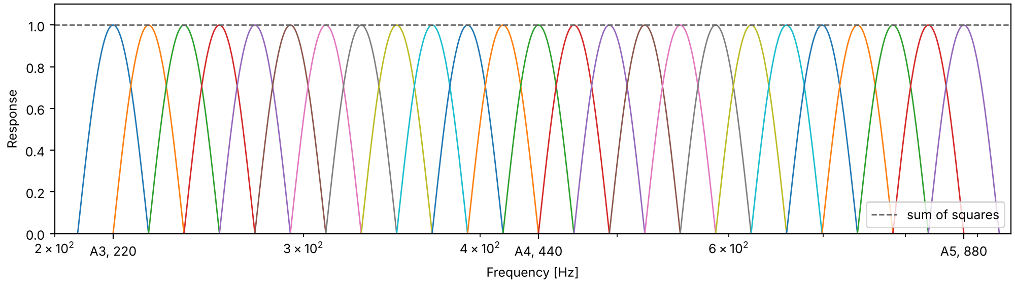
A constant-Q filter bank splits a sound into bands whose width is a fixed fraction of their center frequency (Brown, 1991), so each band spans the same musical interval wherever it sits. sonore's cosine filter bank on the cents scale is one: with a spacing of 100 cents it has one band per semitone. Each band is half a cycle of a cosine over log frequency, zero at its neighbors' centers, so a tone at a band's center reaches that band alone, and the squares of all the responses add up to one at every frequency. Its half-power points lie a quarter tone either side of the center, so its Q, the center frequency over the half-power bandwidth, is 1/(2^{1/24} - 2^{-1/24}), about 17.3 for every band. Because the squares add up to one, filtering each band a second time and adding the bands gives the sound back exactly. The cell measures both on noise. The price is size: every band keeps every sample, so the bank holds one number per band for each sample of the sound.

Code
bank = so.cosine_filterbank(f_lo=55, f_hi=7040, scale="cents", spacing=100)
noise = so.gaussian_noise(2.0, FS, rng=0)
back = bank.synthesize(bank.analyze(noise))
error = np.linalg.norm(back.data - noise.data) / np.linalg.norm(noise.data)
print(f"{bank.n_bands} bands, one per semitone from {bank.band_cfs[0]:.1f} to {bank.band_cfs[-1]:.0f} Hz")
print(f"Q from the formula: {1 / (2 ** (1 / 24) - 2 ** (-1 / 24)):.2f}")
print(f"analyze then synthesize, 2 s of noise: relative error {error:.1e}")
83 bands, one per semitone from 58.3 to 6645 Hz
Q from the formula: 17.31
analyze then synthesize, 2 s of noise: relative error 3.7e-16

The semitone bands from A3 to A5

The responses of the bands from A3 to A5, each a half cycle of a cosine over log frequency. On a logarithmic frequency axis every band has the same width and shape; the dashed line is the sum of their squares, which is one.

The semitone bands from A3 to A5
Code
freqs = np.geomspace(200, 950, 2000)
responses = bank.filter_type.responses(bank, freqs)[:, 1:-1]
shown = (bank.band_cfs >= 219) & (bank.band_cfs <= 881)
fig, ax = plt.subplots(figsize=(10, 2.8), layout="constrained")
ax.plot(freqs, responses[:, shown], lw=1)
ax.plot(freqs, np.sum(responses**2, axis=1), "--", color="0.4", lw=1, label="sum of squares")
ax.set(xscale="log", xlabel="Frequency [Hz]", ylabel="Response", xlim=(200, 950), ylim=(0, 1.1))
ax.set_xticks([220, 440, 880], ["A3, 220", "A4, 440", "A5, 880"])
ax.legend(loc="lower right")

Folding the octaves

Chroma (Fujishima, 1999, who called it a pitch class profile) adds the bands of each pitch class together: C2, C3, C4 and every other C make one row. What is left is the power in each of the twelve pitch classes in each time window. It drops octave height, and with it everything that tells two voicings of a chord apart. It also counts overtones as notes: the third harmonic of C is a G, and its fifth an E, 14 cents flat. The cell prints how the power of the close C major chord below is shared out.

Code
close = [so.note_to_freq(note) for note in ("C4", "E4", "G4")]
spread = [so.note_to_freq(note) for note in ("C3", "G3", "E5")]
chord = sum(harmonic_tone(f0, 2.0) for f0 in close)
power = so.chroma(chord).power[4:-4, :, 0].mean(axis=0)
order = np.argsort(power)[::-1]
names = so.views.chroma.PITCH_CLASSES
print("share of the power:", ", ".join(f"{names[i]} {power[i] / power.sum():.1%}" for i in order[:5]))
share of the power: G 30.8%, E 30.0%, C 28.9%, B 4.1%, D 3.6%

One chord, two voicings

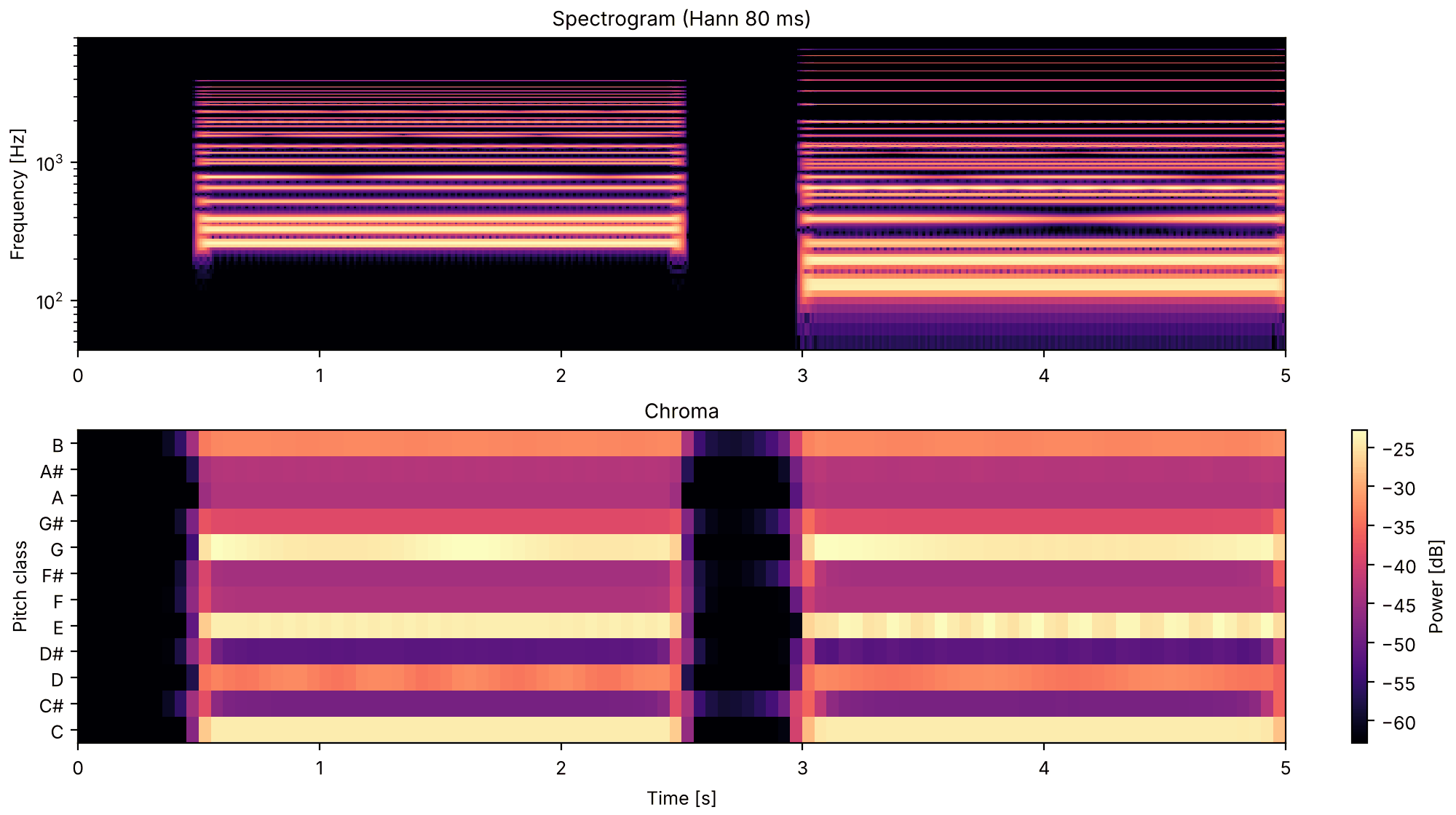
C major, first as C4, E4 and G4 and then spread over three octaves as C3, G3 and E5, two seconds each. The two chords sound different and look different in the spectrogram, but their chroma is much the same: C, E and G, with a little B and D from the overtones.

pc1_one_chord_two_voicings.flac, 5.0 s, mono

Plots of the one chord, two voicings sound
Code
notes = [sum(harmonic_tone(f0, 2.0) for f0 in voicing) for voicing in (close, spread)]
sound = finish(sequence(notes, 2.5))
fig, playhead = show(sound)

Shepard tones

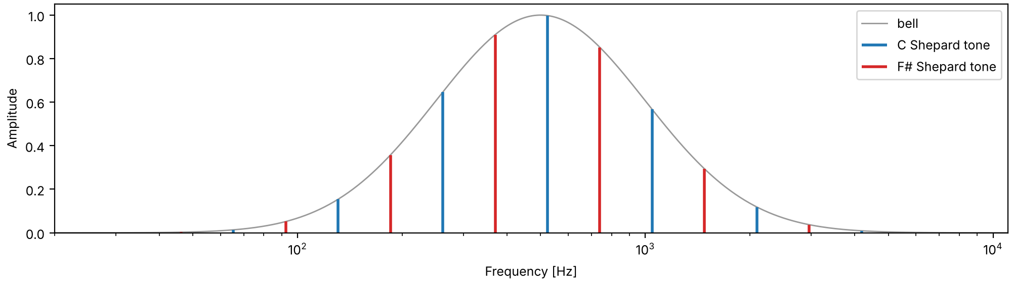
A Shepard tone (Shepard, 1964) is built to have a pitch class and no height. Its partials are an octave apart, so all of them belong to one pitch class, and their levels follow a bell over log frequency that stays put whichever pitch class the tone is. In sonore it is a harmonic complex whose harmonic numbers are powers of two: harmonics=2 ** np.arange(n), with amplitudes the bell. Raise it a semitone and every partial moves up a semitone under the same bell; twelve semitones later every partial sits where its neighbor started, and the tone is the one it began as. The figure shows a C and an F♯.

The partials of two Shepard tones and the bell over them

The partials of two Shepard tones and the bell over them
Code
fig, ax = plt.subplots(figsize=(10, 2.8), layout="constrained")
curve = np.geomspace(20, FS / 2, 400)
ax.plot(curve, bell(0, curve), color="0.6", lw=1, label="bell")
for name, color in [("C4", "C0"), ("F#4", "C3")]:
    freq = so.note_to_freq(name)
    lowest = freq * 2.0 ** -np.ceil(np.log2(freq / 8))
    partials = lowest * 2 ** np.arange(int(np.floor(np.log2(FS / 2 / lowest))) + 1)
    partials = partials[partials >= 20]
    ax.vlines(partials, 0, bell(0, partials), color=color, lw=2, label=f"{name[:-1]} Shepard tone")
ax.set(xscale="log", xlabel="Frequency [Hz]", ylabel="Amplitude", xlim=(20, FS / 2), ylim=(0, 1.05))
ax.legend(loc="upper right")

A scale that keeps rising

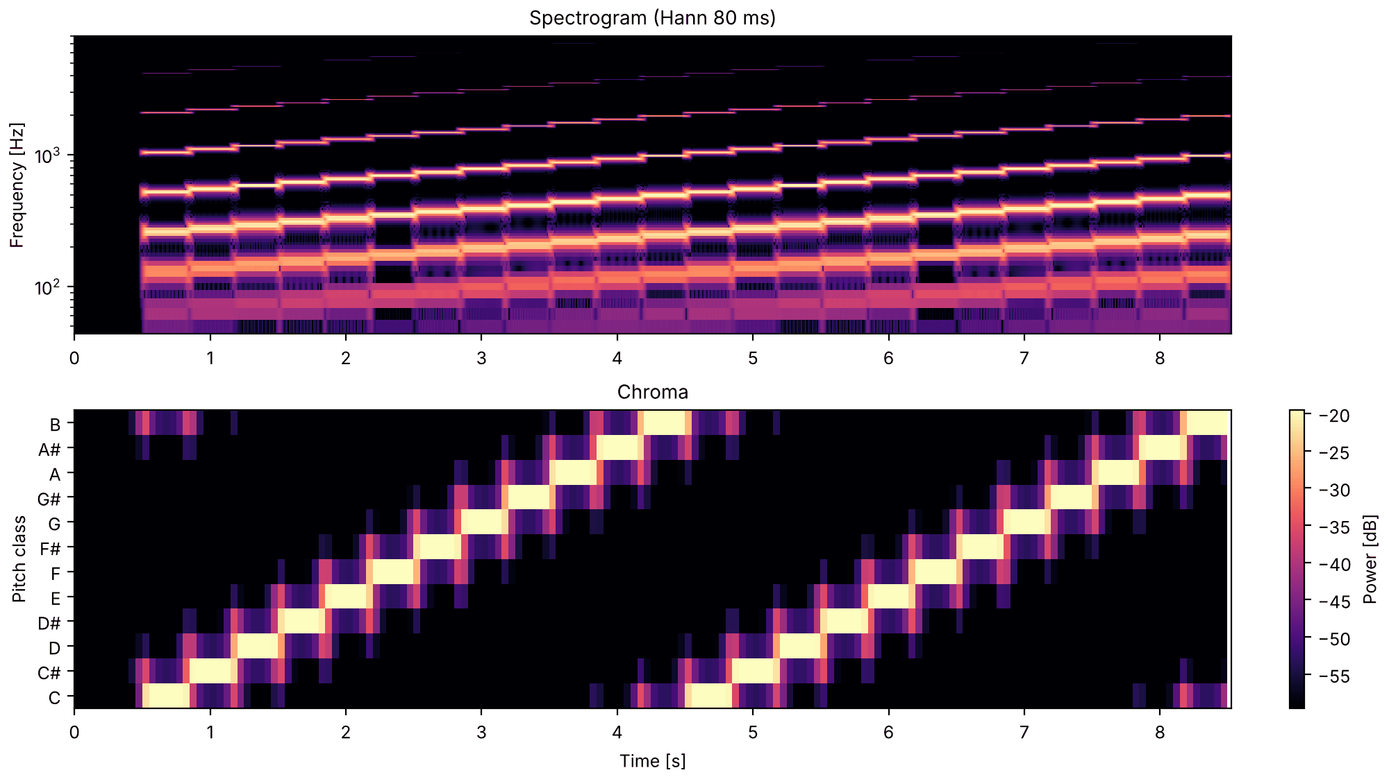
Twenty-four Shepard tones, each a semitone above the last, a third of a second apart: two trips round the twelve pitch classes. Each step is a semitone up; the chroma climbs and starts again, and the bell in the spectrogram does not move.

pc3_a_scale_that_keeps_rising.flac, 8.5 s, mono

Plots of the a scale that keeps rising sound
Code
c4 = so.note_to_freq("C4")
notes = [shepard_tone(c4 * 2 ** (step / 12), 0.36) for step in range(24)]
sound = finish(sequence(notes, 1 / 3))
fig, playhead = show(sound)

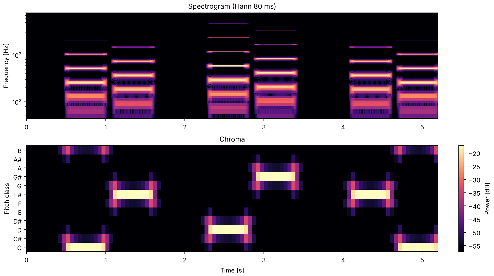
Halfway round, a tritone, is the case with no nearer way to go: up six semitones and down six land on the same pitch class. Listeners asked whether such a pair rises or falls disagree, and the answer depends on which pitch classes the pair uses (Deutsch, 1986): the tritone paradox. Nothing in the spectrum separates the twelve Shepard tones by height; the cell measures the power-weighted mean of log frequency for each. The page makes no claim about how the pairs below sound to any listener.

Code
def mean_octave(snd):
    """The power-weighted mean of log2 frequency [octaves above 1 Hz], from the spectrum."""
    spectrum = np.abs(np.fft.rfft(snd.data[:, 0])) ** 2
    freqs = np.fft.rfftfreq(snd.n_samples, 1 / FS)
    keep = freqs > 0
    return np.sum(spectrum[keep] * np.log2(freqs[keep])) / np.sum(spectrum[keep])


means = [mean_octave(shepard_tone(c4 * 2 ** (step / 12), 1.0)) for step in range(12)]
print(f"mean log2 frequency over the 12 pitch classes: {min(means):.3f} to {max(means):.3f} octaves")
print(f"the bell's center, {BELL_CENTER:g} Hz: {np.log2(BELL_CENTER):.3f} octaves")
mean log2 frequency over the 12 pitch classes: 8.965 to 8.966 octaves
the bell's center, 500 Hz: 8.966 octaves

Two tones a tritone apart

Three pairs of Shepard tones a tritone apart, half a second each: C then F♯, D then G♯, and F♯ then C.

pc4_two_tones_a_tritone_apart.flac, 5.2 s, mono

Plots of the two tones a tritone apart sound
Code
pairs = [("C4", "F#4"), ("D4", "G#4"), ("F#4", "C4")]
notes = []
for first, second in pairs:
    notes += [shepard_tone(so.note_to_freq(first), 0.5), shepard_tone(so.note_to_freq(second), 0.5)]
    notes.append(so.silence(0.5, FS))
sound = finish(sequence(notes[:-1], 0.6))
fig, playhead = show(sound)

The Risset glide

The Shepard scale moves in steps; Risset (1969) made it glide. The recipe is the same harmonic complex with a rising F0 contour instead of a fixed F0. The lowest partial starts five octaves below 20 Hz, so as every partial rises and fades out at the top of the bell, another rises into view from below, and the sound keeps the same spread of partials under the bell throughout. Each partial follows its octave multiple of the contour exactly.

An endless glide upward

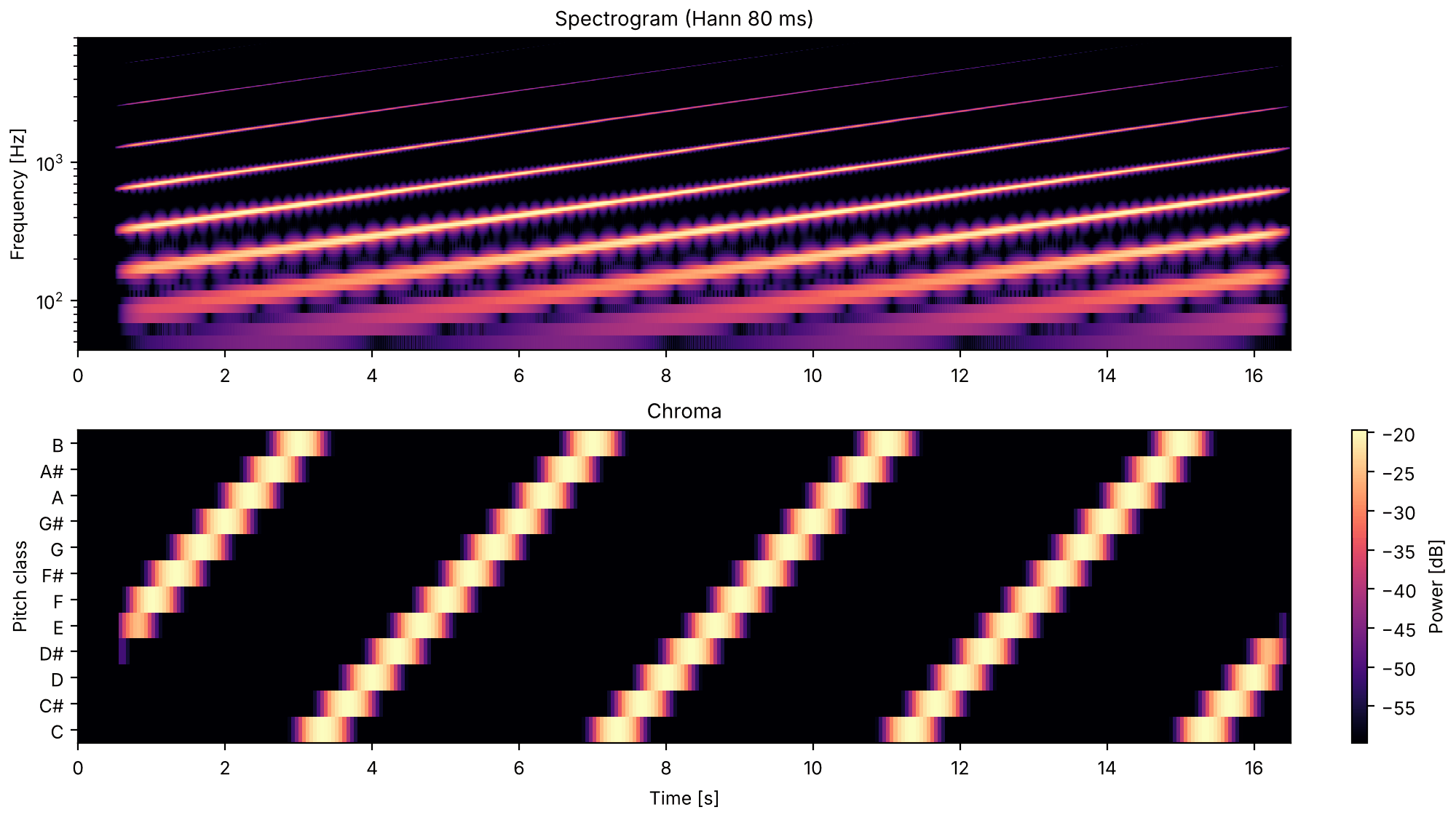
Sixteen seconds of glide, one octave every four seconds: four times round the pitch classes. In the spectrogram the partials climb and the bell stays put; in the chroma one band of power climbs and wraps round.

pc5_an_endless_glide_upward.flac, 16.5 s, mono

Plots of the an endless glide upward sound
Code
duration = 16.0
times = np.linspace(0, duration, 400)
contour = (times, 20 / 2**5 * 2 ** (times / 4))  # one octave every 4 s
octaves = 2 ** np.arange(20)
glide = so.harmonic_complex(duration, FS, contour, harmonics=octaves, amplitudes=bell, f_max=FS / 2)
sound = finish(sequence([glide.ramp(0.5)], 0))
fig, playhead = show(sound)

Back from chroma

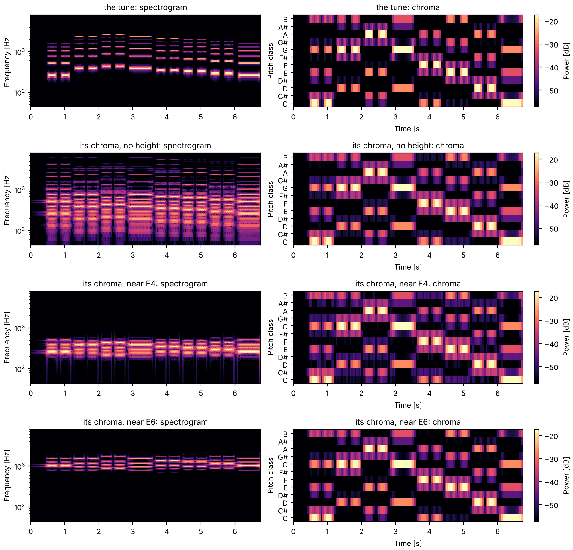
Chroma cannot be inverted: many sounds share it. What it dropped is how each pitch class's power spreads across the octaves, and Chroma.to_sound takes exactly that as its argument, octaves. By default it plays each pitch class as a Shepard tone, with a bell centered between the lowest and highest band (A1 and A8) and one octave wide. A Shepard tone's partials are all octaves of one pitch class, so its chroma comes back unchanged; a harmonic tone could not do that, since its overtones land on other pitch classes. Given a note such as "E4", the bell is narrow and centered there, and each pitch class sounds in the octave nearest that note. The tune below runs from C4 to A4, all within half an octave of E4, so near E4 its notes come back in their own octave, and near E6 two octaves up.

A note that starts or stops is no longer a steady tone at one band's center, so for a moment it splashes a little power into the neighboring semitones, its overtones included. Chroma keeps that splash, and played back it sounds like a grace note a semitone away. The gentler the change, the smaller the splash: here each note fades in and out over 60 ms. The same semitone-wide bands also blur timing: a band one semitone wide keeps ringing for tens of milliseconds after its tone stops (longer for lower notes), so a silence between notes comes back shallower and shorter than it went in. The tune is played detached, with 150 ms of silence after each note, so that repeated notes stay apart in the playback. Its notes have six harmonics, not ten: the seventh harmonic lies 31 cents below an equal-tempered pitch class, and played back as that pitch class it sounds out of tune with the rest. The first six land on the note, its fifth and its major third. The cell compares the chroma of each sound below with the tune's.

Code
# The first two lines of Twinkle, Twinkle, Little Star, as (note, beats); each line ends on a
# note held for two beats.
TUNE = [
    ("C4", 1),
    ("C4", 1),
    ("G4", 1),
    ("G4", 1),
    ("A4", 1),
    ("A4", 1),
    ("G4", 2),
    ("F4", 1),
    ("F4", 1),
    ("E4", 1),
    ("E4", 1),
    ("D4", 1),
    ("D4", 1),
    ("C4", 2),
]
BEAT, GAP = 0.4, 0.15  # a beat, and the silence after each note [s]
melody = sequence(
    [
        harmonic_tone(so.note_to_freq(note), beats * BEAT - GAP, fade=0.06, partials=np.arange(1, 7))
        for note, beats in TUNE
    ],
    [beats * BEAT for _, beats in TUNE],
)
melody_chroma = so.chroma(melody)
played = {
    "the tune": melody,
    "its chroma, no height": melody_chroma.to_sound(FS),
    "its chroma, near E4": melody_chroma.to_sound(FS, octaves="E4"),
    "its chroma, near E6": melody_chroma.to_sound(FS, octaves="E6"),
}
for label, snd in played.items():
    measured = so.chroma(snd).power[:, :, 0]
    shares = measured.sum(axis=0) / measured.sum()
    reference = melody_chroma.power[:, :, 0].sum(axis=0) / melody_chroma.power.sum()
    difference = np.abs(shares - reference).max()
    print(f"{label:24s} largest difference in a pitch class's share of the power: {difference:.4f}")
the tune                 largest difference in a pitch class's share of the power: 0.0000
its chroma, no height    largest difference in a pitch class's share of the power: 0.0014
its chroma, near E4      largest difference in a pitch class's share of the power: 0.0047
its chroma, near E6      largest difference in a pitch class's share of the power: 0.0004

A tune and its chroma played back

The tune, then its chroma played three ways: as Shepard tones with no height, and with the bell narrowed to the octaves near E4 and near E6. The three have the tune's chroma; they differ in what the chroma dropped. The chroma of the original includes its overtones, so the Shepard tones play those pitch classes too, quietly. The chroma keeps one value per 50 ms time window, so each note of the playback starts and stops over about that long, and the splash at each change of note is still there, softly.

the tune

pc6_a_tune_and_its_chroma_played_back_the_tune.flac, 6.7 s, mono

its chroma, no height

pc6_a_tune_and_its_chroma_played_back_its_chroma_no_height.flac, 6.7 s, mono

its chroma, near E4

pc6_a_tune_and_its_chroma_played_back_its_chroma_near_e4.flac, 6.7 s, mono

its chroma, near E6

pc6_a_tune_and_its_chroma_played_back_its_chroma_near_e6.flac, 6.7 s, mono

Plots of the a tune and its chroma played back sounds
Code
sounds = {label: finish(snd) for label, snd in played.items()}
fig = plt.figure(figsize=(10, 9.6), layout="constrained")
rows = fig.subfigures(len(sounds), 1)
playhead = {}
for row, (label, snd) in zip(rows, sounds.items(), strict=True):
    ax_spectrogram, ax_chroma = row.subplots(1, 2)
    draw(snd, ax_spectrogram, ax_chroma)
    ax_spectrogram.set_title(f"{label}: spectrogram")
    ax_chroma.set_title(f"{label}: chroma")
    playhead[label] = [ax_spectrogram, ax_chroma]

References

  • Brown (1991). Calculation of a constant Q spectral transform. J. Acoust. Soc. Am. 89(1), 425–434. doi:10.1121/1.400476.
  • Deutsch (1986). A musical paradox. Music Perception 3(3), 275–280. doi:10.2307/40285337.
  • Fujishima (1999). Realtime chord recognition of musical sound: a system using Common Lisp Music. Proc. International Computer Music Conference, 464–467. CCRMA abstract.
  • Risset (1969). Pitch control and pitch paradoxes demonstrated with computer-synthesized sounds. J. Acoust. Soc. Am. 46, 88 (abstract). doi:10.1121/1.1973626.
  • Shepard (1964). Circularity in judgments of relative pitch. J. Acoust. Soc. Am. 36(12), 2346–2353. doi:10.1121/1.1919362.