A sound texture is made of many similar events. This page builds one from a single event with
so.event_train, then measures the events of a real texture, a fire's pops, and what a
synthesis from the texture model of Sound textures keeps of them.
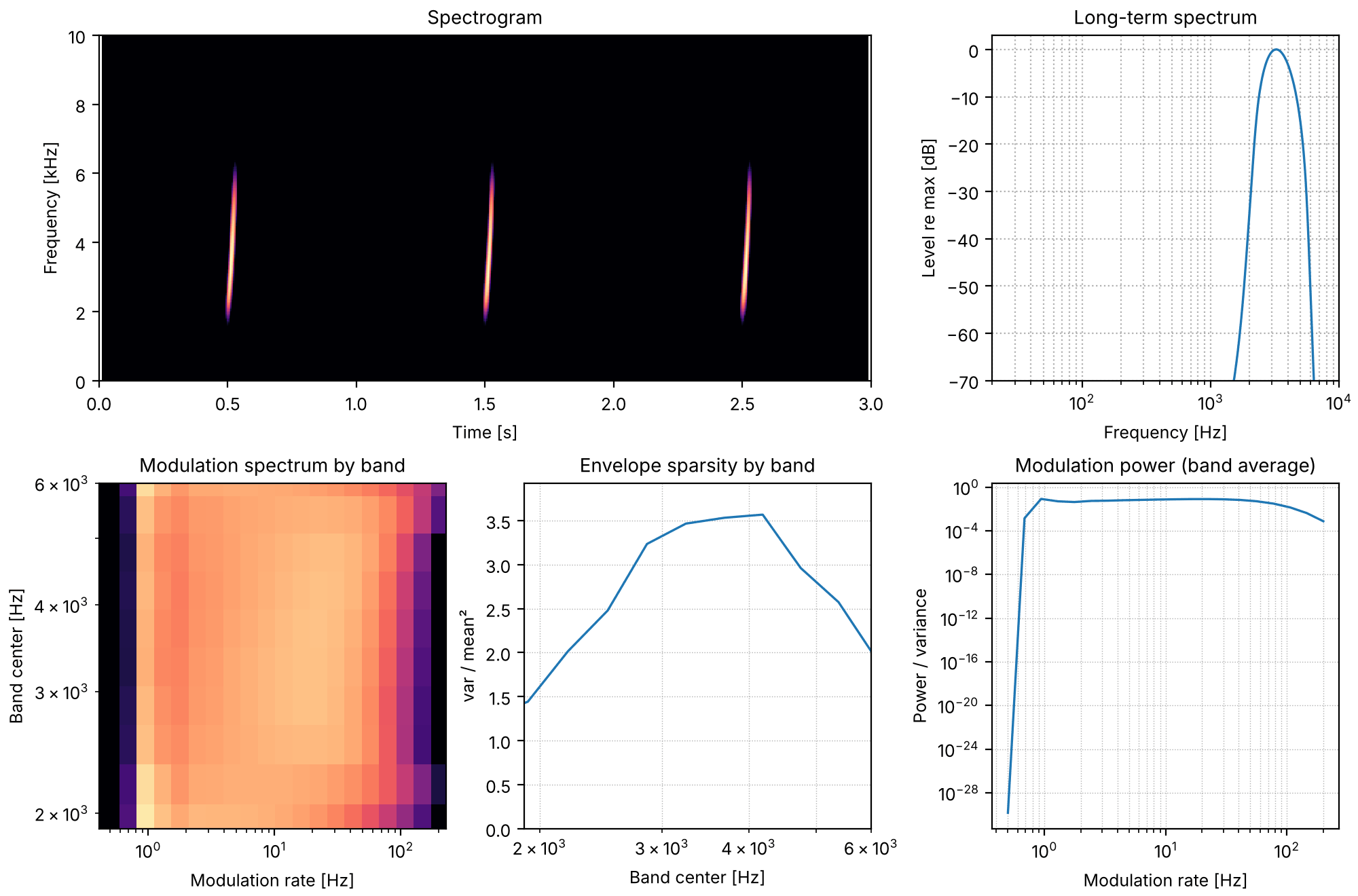
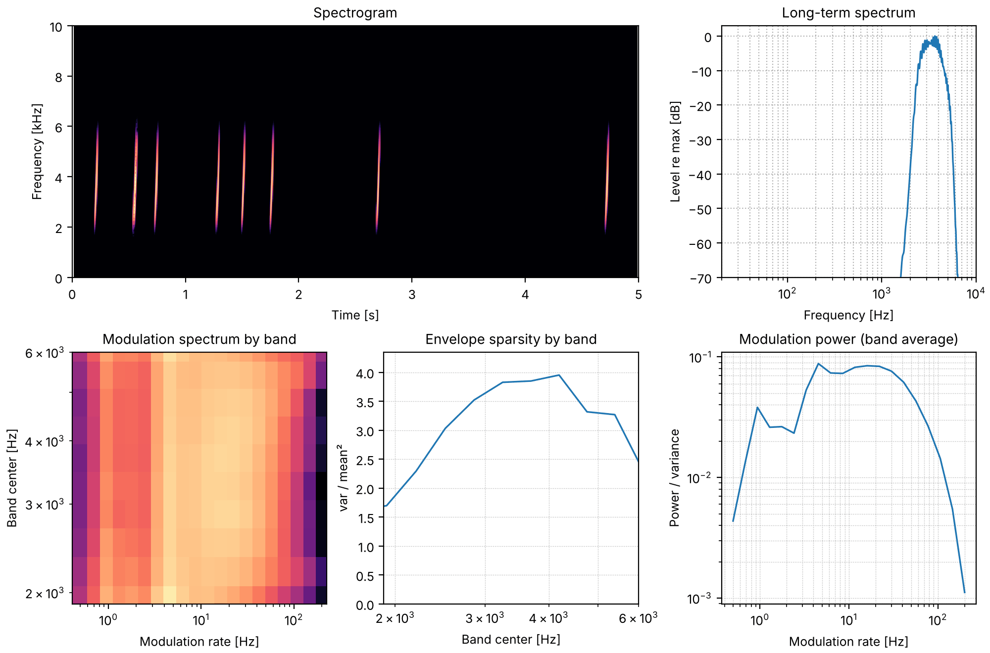
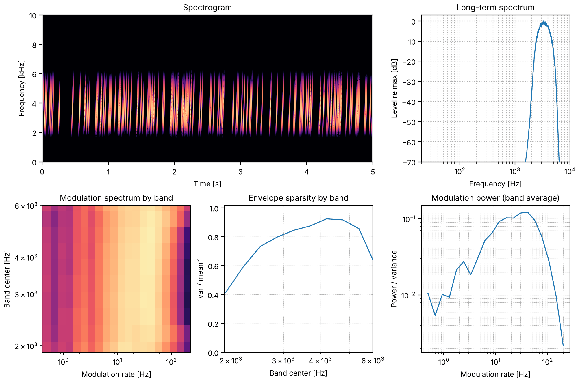
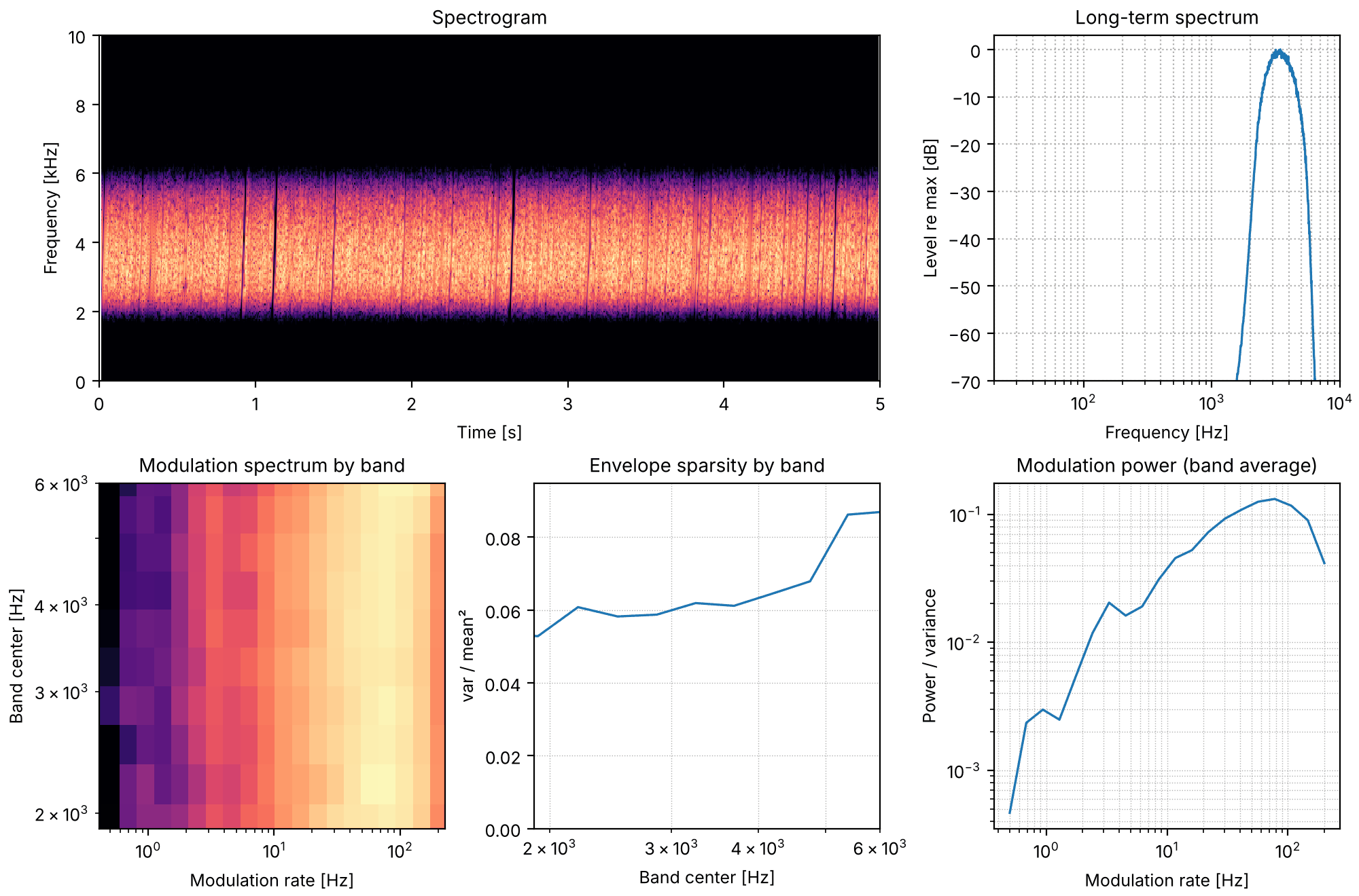
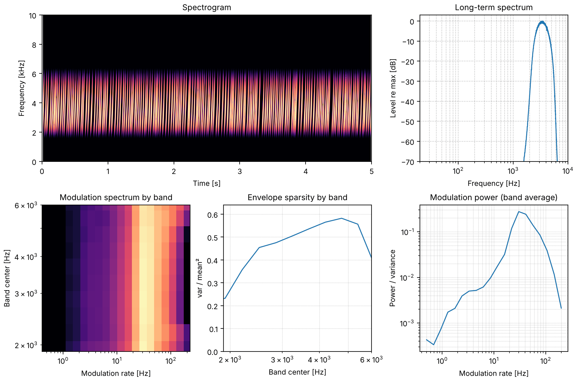
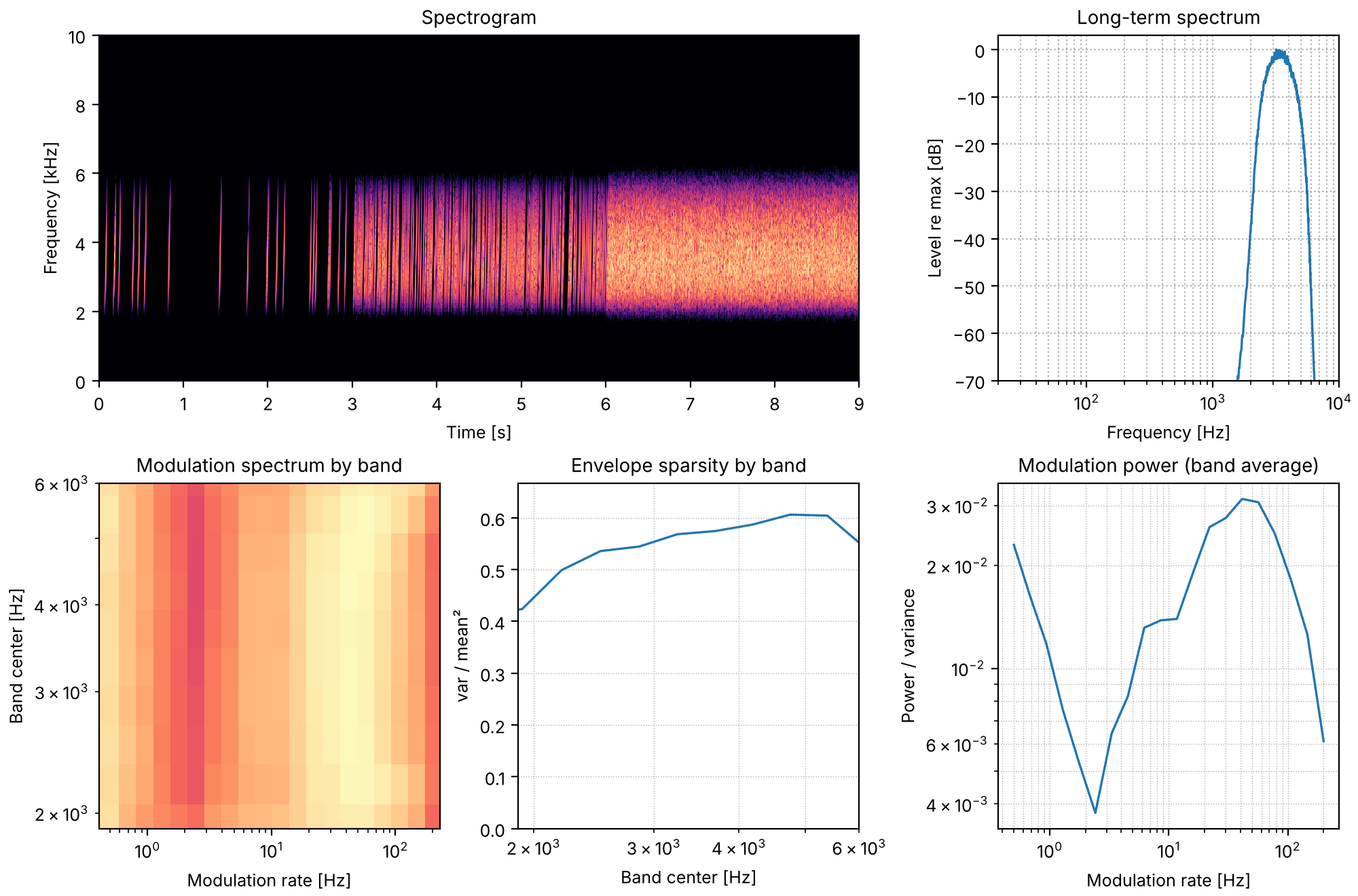
From single events to a texture: one chirp copied at rising rates, from events that stand apart to a dense sum, and what level, pitch and timing spreads do.
How big the pops are: the sizes of a fire's pops follow a power law, measured by its exponent, and what a synthesis keeps of it.
Press play and a line follows the sound across every time axis in its plots. Click any time
axis to play from that point. Start with your volume low.
To run this page yourself, open it as a notebook in Colab or download it. It is the same code, and it fetches the recordings it needs from the sonore repository.
Code the examples share
Every example below is the code shown with it, run after this cell: loading a recording and
its synthesis, the level the gallery plays sounds at, and the plots of the texture model's
statistics, the same as on Sound textures.
Setup, the same on every page
import os
import urllib.request

import matplotlib.pyplot as plt
import numpy as np

import sonore as so

plt.rcParams.update({"font.size": 9, "axes.titlesize": 10, "figure.dpi": 100})


def fetch(path):
    """A file from the sonore repository, by its path there: the local copy when this runs from
    the repository root, otherwise downloaded from GitHub to the same relative path."""
    if not os.path.exists(path):
        os.makedirs(os.path.dirname(path) or ".", exist_ok=True)
        urllib.request.urlretrieve("https://raw.githubusercontent.com/choyun1/sonore/main/" + path, path)
    return path


def finish(snd):
    """How every sound in the gallery is played: 5 ms ramps, RMS 0.1, peak at most 0.95."""
    snd = snd.ramp(5e-3).normalize(rms=0.1)
    return snd.normalize(peak=0.95) if snd.peak > 0.95 else snd
Code
import json

from sonore.texture import TextureStats

FS = 44100


def original(name):
    """A recording; docs/textures/SOURCES.md says where each comes from and which excerpt."""
    return so.load(fetch(f"docs/textures/{name}.flac"))


def synthesized(name, imposed=""):
    """A synthesis precomputed by tools/make_texture_synths.py (below)."""
    suffix = f"__{imposed}" if imposed else ""
    return so.load(fetch(f"docs/textures/synth/{name}{suffix}.flac")).resample(FS)


def report(name):
    """How closely the synthesis matches: the statistic SNR averaged over classes."""
    info = json.loads(open(fetch(f"docs/textures/synth/{name}.json")).read())
    snr = np.mean(list(info["snr_all_classes"].values()))
    return f"Average statistic SNR {snr:.0f} dB after {info['best_iteration']} iterations."


def texture_fig(snd, original, synthetic=False):
    """General-purpose plots (spectrogram, long-term spectrum) plus the texture
    model's own statistics drawn with plain matplotlib: modulation power by
    band and rate (the model's modulation spectrum), envelope sparsity, and
    band-averaged modulation power. Dashed black: the original."""
    fig = plt.figure(figsize=(10, 6.6), layout="constrained")
    gs = fig.add_gridspec(2, 3)
    ax_s = fig.add_subplot(gs[0, :2])
    ax_l, ax_m, ax_v, ax_p = (fig.add_subplot(gs[r, c]) for r, c in ((0, 2), (1, 0), (1, 1), (1, 2)))
    so.STFT(snd, win_dur=20e-3).plot(ax_s, fmax=10000, db_range=70, colorbar=False)
    ax_s.set_title("Spectrogram")
    so.long_term_spectrum(snd).plot(ax_l, lw=1.2, label="this sound")
    if synthetic:
        so.long_term_spectrum(original).plot(ax_l, color="k", ls="--", lw=1, label="original")
        ax_l.legend(fontsize=7)
    ax_l.set(xlim=(20, 10000), ylim=(-70, 3), title="Long-term spectrum")
    target = TextureStats.measure(original)
    this = TextureStats.measure(snd, window="uniform" if synthetic else "ramped")  # syntheses are circular
    cfs = target.model.filterbank.cfs[1:-1]
    ok = target.channel_mask()
    # The model's modulation spectrum: power at each modulation rate, in each cochlear band.
    mcf = target.model.mod_bank.cfs
    lev = 10 * np.log10(np.maximum(this.mod_power[1:-1], 1e-6))
    ax_m.pcolormesh(mcf, cfs, lev, cmap="magma", vmin=lev.max() - 25, vmax=lev.max(), shading="nearest")
    ax_m.set(
        xscale="log",
        yscale="log",
        xlabel="Modulation rate [Hz]",
        ylabel="Band center [Hz]",
        title="Modulation spectrum by band",
    )
    ax_v.semilogx(cfs, this.env_var[1:-1], lw=1.2)
    ax_p.loglog(target.model.mod_bank.cfs, this.mod_power[ok].mean(0), lw=1.2)
    if synthetic:
        ax_v.semilogx(cfs, target.env_var[1:-1], "k--", lw=1)
        ax_p.loglog(target.model.mod_bank.cfs, target.mod_power[ok].mean(0), "k--", lw=1)
    ax_v.set(xlabel="Band center [Hz]", ylabel="var / mean²", title="Envelope sparsity by band")
    ax_p.set(
        xlabel="Modulation rate [Hz]", ylabel="Power / variance", title="Modulation power (band average)"
    )
    for ax in (ax_v, ax_p):
        ax.grid(ls=":", which="both", lw=0.5)
    return fig, [ax_s]  # the playhead follows the spectrogram
From single events to a texture
A texture, by the definition on Sound textures, is many similar events, and
that can be built directly. so.event_train copies one
event at onsets whose intervals are drawn from a distribution, here exponential, which makes
the onsets a Poisson process. Its long-term spectrum is the event's own at every rate; what the
rate changes is how many events overlap, and with it the statistics beyond the spectrum (the
design notes measure both: event-texture.md).
Code
from scipy import stats

chirp = so.exponential_chirp(0.03, FS, 2000, 6000)
chirp = chirp * np.hanning(len(chirp))[:, None]


def chorus(rate, duration=5.0, seed=0, **kwargs):
    """Copies of the chirp at Poisson onsets, `rate` per second on average."""
    return so.event_train(chirp, duration, stats.expon(scale=1 / rate), lead=0.03, rng=seed, **kwargs)


def events_fig(snd):
    """The same plots as the recordings on Sound textures, measured on this sound alone. The panels by band
    show only the bands from 2 to 6 kHz, where the chirp has its energy: elsewhere the
    statistics are those of numerical noise."""
    fig, playhead = texture_fig(snd, snd)
    _, _, ax_m, ax_v, _ = fig.axes
    band_centers, sparsity_by_band = ax_v.lines[0].get_data()
    in_band = (band_centers >= 2000) & (band_centers <= 6000)
    ax_v.set(xlim=(1900, 6000), ylim=(0, 1.1 * sparsity_by_band[in_band].max()))
    ax_m.set_ylim(1900, 6000)
    return fig, playhead
The event
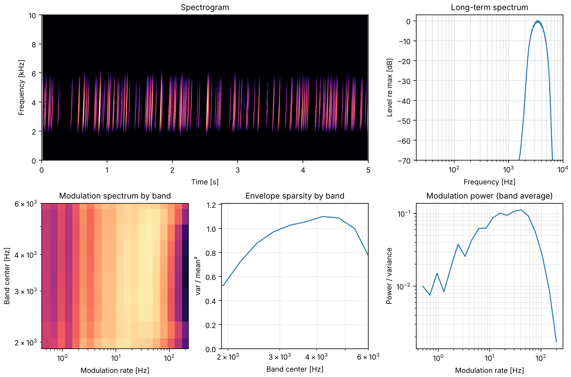
The event: a 30 ms sweep from 2 to 6 kHz, exponential in frequency, under a Hann window,
repeated once a second here so it can be heard on its own.
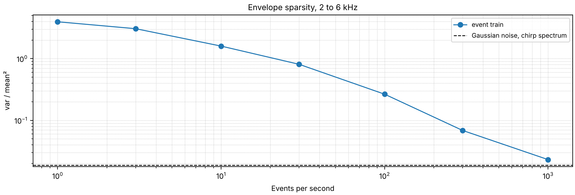
Where each rate sits on one of the texture model's statistics: the envelope variance over the
squared mean (env_var, as in the plots above), averaged over the bands from 2 to 6 kHz where
the chirp has its energy, measured on 10 s of each rate. The dashed line is Gaussian noise
filtered to the chirp's spectrum, the limit as the rate grows. This is a one-way view: it
places each sound on one statistic and says nothing about its rhythm or onsets.
Each copy's level and pitch can be drawn from a distribution too, and so can the timing. All
examples below are at 30 events per second, the rate where events start to run into each
other. A spread in level leaves a few loud events standing out of the rest, which keeps the
sound sparse by the measure above for longer as the rate rises; a spread in pitch widens the
spectrum. Nearly regular timing puts a steady rhythm at the rate into the envelope.
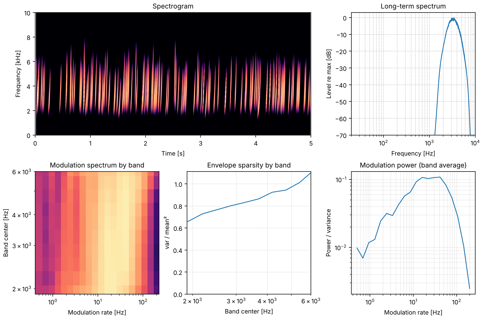
Level spread, 9 dB
Levels drawn from a normal distribution in dB, standard deviation 9 dB.
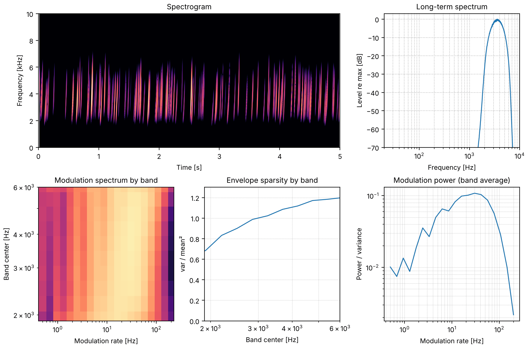
Both spreads at once: levels with a standard deviation of 9 dB and pitch shifts with a standard
deviation of 150 cents, drawn independently for each copy.
Intervals from a gamma distribution with shape 16: the same mean rate, but intervals vary by
only a quarter of their mean, so the events come almost evenly.
A rate that changes over time: rate_scale steps from 10 to 100 and 1000 events per second,
3 s at each. A track is interpolated linearly between its points, so each step is written as
two points a microsecond apart.
and infinite for n \ge \alpha: the variance needs \alpha > 2 and the kurtosis \alpha > 4.
Below that, a moment measured on a recording keeps growing with the recording's length, because
a longer recording catches rarer, bigger pops: over 1 s pieces of the fire recording the
envelope kurtosis is about 220, over all 20 s about 1900. The texture model describes each band
by such moments, so for a sound like this it matches numbers that belong to the excerpt more
than to the sound. The exponent does not drift. From the k largest values,
x_{(1)} \ge x_{(2)} \ge \dots \ge x_{(k+1)}, the Hill estimator is
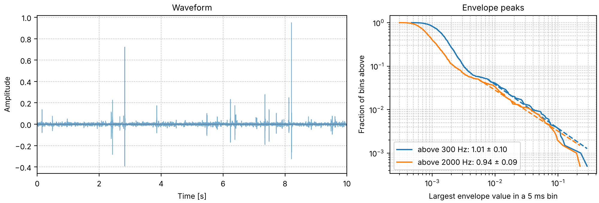
with a standard error of about \hat\alpha / \sqrt{k}. so.envelope_peaks applies it to the
largest envelope value in each 5 ms bin of the sound high-passed at 300 Hz and at 2 kHz,
fitting the largest 5%. Below about 2 a sound is made of pops; of the recordings on Sound
textures, the stream gives about 3, the rain about 5 and the crickets about
10. The design notes give the measurement, how far to trust it, and a survey of the 168
recordings of McDermott & Simoncelli (2011):
envelope-peaks.md.
Envelope peaks of the fire and its synthesis
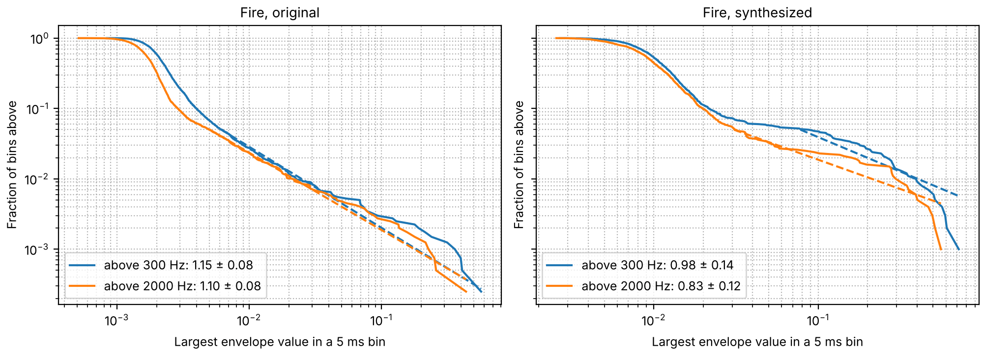
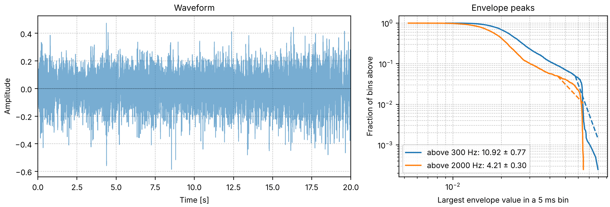
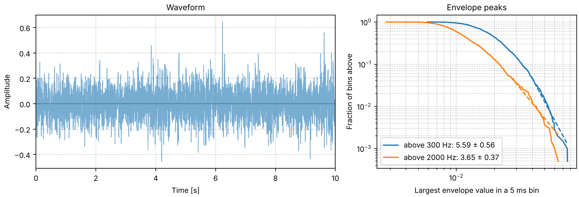
The fraction of 5 ms bins whose largest envelope value exceeds each value, on log-log axes,
for the fire recording (20 s) and its synthesis (5 s). A power law is a straight line here, with
slope -\alpha; the dashed lines are the fits. The original is close to a straight line over
almost two decades. The synthesis gets about the same exponent from its largest 5%, but its
curve is not straight: a shelf of medium-sized peaks, then a steep drop. Its loud moments come
in a narrower range of sizes, which the single number misses and the curve shows.
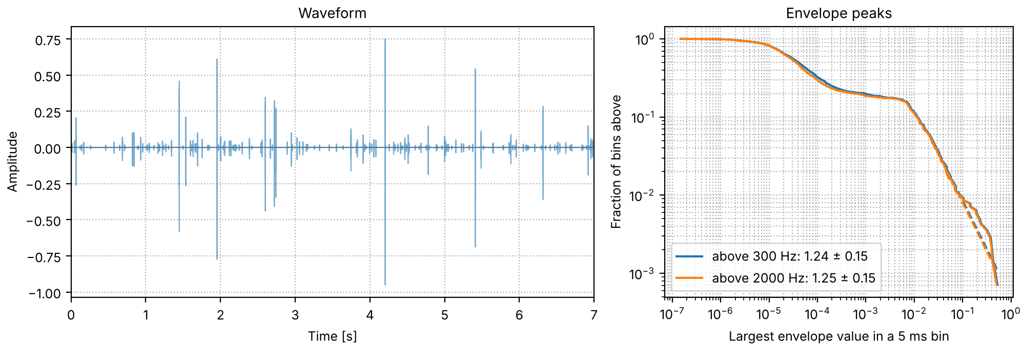
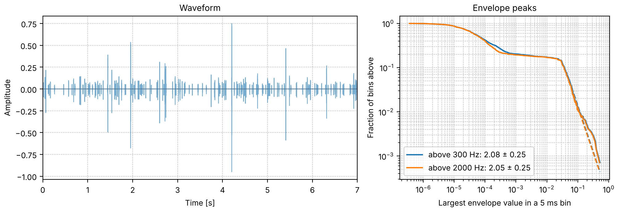
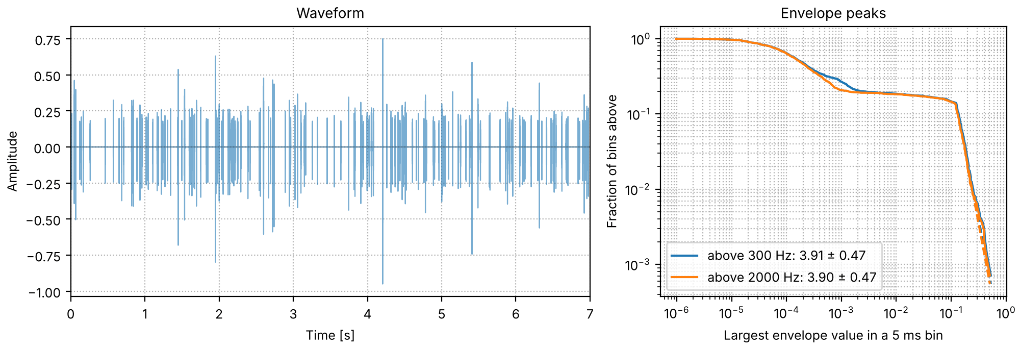
To hear what the exponent means, so.event_train can make pops whose sizes follow a power law
with a chosen exponent. A pop's level in dB above the smallest, L = 20 \log_{10}(A / x_0), has
P(L > l) = e^{-l \alpha \ln 10 / 20}: power-law sizes are exponentially distributed levels, with
scale 20 / (\alpha \ln 10) dB. Below, a 3 ms burst of noise,
30 times a second on average, with levels capped at 40 dB above the smallest. The exponent
measured on each comes out close to the one asked for.
Code
burst = so.gaussian_noise(0.003, FS, rng=0)
burst = burst * np.hanning(len(burst))[:, None]


def pops(exponent, rate=30, duration=7.0, seed=0):
    """Bursts at Poisson onsets, with levels whose amplitudes follow a power law."""
    scale = 20 / (exponent * np.log(10))  # dB
    levels = stats.truncexpon(b=40 / scale, scale=scale)  # 0 to 40 dB
    return so.event_train(burst, duration, stats.expon(scale=1 / rate), level_db=levels, lead=0.01, rng=seed)


def pops_fig(snd):
    """The waveform, and the envelope peaks as above."""
    fig, (ax_wave, ax_peaks) = plt.subplots(
        1, 2, figsize=(10, 3.4), layout="constrained", gridspec_kw={"width_ratios": [3, 2]}
    )
    snd.plot(ax_wave)
    so.envelope_peaks(snd).plot(ax_peaks)
    return fig, [ax_wave]
Pops, exponent 1
Exponent 1: most pops are small, and every few seconds one is far louder than the rest.
The fire's synthesis keeps pops, but too many of them are medium-sized, and the background
sits too close to the biggest: the median bin is 35 dB below the biggest pops in the
synthesis, 43 dB in the original. A synthesis as long as the original does no better. What
sounded closer to the original by ear was to take the pops out, synthesize the rest, and put
pops back with so.event_train:
Remove the pops. Scale each 5 ms bin so that its largest envelope value is at most twice the 80th percentile of those values, with the gain smoothed over 2 ms.
Synthesize the background. Without its pops the fire is an ordinary texture, and the model matches it well (39 dB average statistic SNR, against 21 dB for the whole fire).
Add pops. The recording's eight biggest pops, 15 ms each, as events at Poisson onsets at the rate pops cross the threshold in the original, with power-law levels at the exponent measured on the original, from the threshold up to the biggest pop. The background goes 3 dB down, which sounds closer to the original than leaving it as it is.
This recipe is sonore's own, put together for this page from standard parts (texture
synthesis, and shot noise with power-law sizes); we know of no paper that describes it, and it
is not a validated method. Its only test is one listener comparing it by ear with the plain
synthesis on a handful of the paper's recordings. There it sounded closer on two other fires
and a clapper close to the microphone, pops that are random in time over a steady background,
and no better on rhythmic or impact sounds (tapping, a bongo loop, a typewriter, castanets),
which the texture model also synthesizes poorly on its own; McDermott & Simoncelli (2011) list
rhythm among the model's failures.
Code
def remove_pops(sound):
    """The sound with its pops limited away: each 5 ms bin is scaled so that its largest envelope
    value above 300 Hz is at most twice the 80th percentile of those values. The gain is
    smoothed over 2 ms so the cuts do not click. tools/make_texture_synths.py synthesizes the
    fire's background with this same function."""
    peaks = so.envelope_peaks(sound, cutoffs_hz=(300.0,))
    maxima = peaks.maxima[:, 0]
    threshold = 2 * np.percentile(maxima, 80)
    bin_length = int(round(peaks.bin_seconds * sound.fs))
    gain = np.ones(len(sound))
    gain[: len(maxima) * bin_length] = np.repeat(np.minimum(1.0, threshold / maxima), bin_length)
    smoothing = np.hanning(int(0.002 * sound.fs))
    gain = np.minimum(gain, np.convolve(gain, smoothing / smoothing.sum(), "same"))
    return sound * gain[:, None]


def biggest_pops(sound, count=8, length=0.015):
    """The `count` biggest pops, each `length` long from 2 ms before its peak, at least 0.1 s apart,
    with softened edges and unit peak."""
    peaks = so.envelope_peaks(sound, cutoffs_hz=(300.0,))
    maxima = peaks.maxima[:, 0]
    chosen = []
    for bin_index in np.argsort(maxima)[::-1]:
        if all(abs(bin_index - other) * peaks.bin_seconds > 0.1 for other in chosen):
            chosen.append(bin_index)
        if len(chosen) == count:
            break
    samples, fs = sound.data[:, 0], sound.fs
    bin_length = int(round(peaks.bin_seconds * fs))
    n_event = int(length * fs)
    events = []
    for bin_index in chosen:
        in_bin = samples[bin_index * bin_length : (bin_index + 1) * bin_length]
        start = max(bin_index * bin_length + int(np.argmax(np.abs(in_bin))) - int(0.002 * fs), 0)
        piece = samples[start : start + n_event] * np.hanning(n_event) ** 0.25
        events.append(so.Sound(piece / np.abs(piece).max(), fs))
    return events


def background_plus_pops(sound, background, background_db=-3.0, seed=0):
    """`background` (a synthesis of `remove_pops(sound)`) with pops from `sound` added: the rate, the
    exponent and the range of sizes are measured on `sound`, the smallest pop sits at the
    threshold `remove_pops` limits to, and the background is `background_db` down."""
    peaks = so.envelope_peaks(sound, cutoffs_hz=(300.0,))
    maxima = peaks.maxima[:, 0]
    threshold = 2 * np.percentile(maxima, 80)
    rate = np.sum((maxima[1:] > threshold) & (maxima[:-1] <= threshold)) / sound.duration
    range_db = 20 * np.log10(maxima.max() / threshold)
    scale = 20 / (peaks.exponent[0] * np.log(10))  # dB
    levels = stats.truncexpon(b=range_db / scale, scale=scale)
    events = biggest_pops(sound)
    out = background * 10 ** (background_db / 20)
    for k, event in enumerate(events):
        size = so.envelope_peaks(event.pad(0.05, 0.05), cutoffs_hz=(300.0,)).maxima.max()
        train = so.event_train(event * (threshold / size), background.duration,
                               stats.expon(scale=len(events) / rate), level_db=levels, rng=seed + k)
        out = out + train[: background.duration]
    return out


fire = original("fire")
fire_background = synthesized("fire", "background")
fire_background = fire_background * (remove_pops(fire).rms / fire_background.rms)
Fire with its pops removed
The fire with its pops limited away: the hiss and rumble under the pops.
The synthesized background, 3 dB down, with the recording's own pops added back at power-law
sizes. Compare with the original and the synthesis on Sound textures.
Hill (1975). A simple general approach to inference about the tail of a distribution. Annals of Statistics 3(5), 1163–1174. doi:10.1214/aos/1176343247. envelope_peaks
McDermott & Simoncelli (2011). Sound texture perception via statistics of the auditory periphery. Neuron 71(5), 926–940. doi:10.1016/j.neuron.2011.06.032. texture