Two talkers

Every page about speech in this gallery uses one sentence, "Providence had delivered him through the maelstrom," read by two talkers from the CMU ARCTIC corpus (Kominek and Black, 2004): a male talker (speaker bdl) and a female talker (speaker slt), both recorded at 16 kHz. Each analysis is shown on both, because what an analysis gets right on one voice it can get wrong on another, and the most common reason is pitch.

This page measures how the two recordings differ, once, so that the other pages can refer to it. Each talker is one person: the numbers describe these two recordings, not men and women in general. Where a page needs averages over many talkers, it cites them.

Press play and a line follows the sound across every time axis in its plots. Click any time axis to play from that point. Start with your volume low.

To run this page yourself, open it as a notebook in Colab or download it. It is the same code, and it fetches the recordings it needs from the sonore repository.

The sentence, read twice

The code every speech page starts from: the two recordings, each with the pitch track that so.f0_track measures (see Pitch tracking), and a figure with one column per talker.

Setup, the same on every page
import os
import urllib.request

import matplotlib.pyplot as plt
import numpy as np

import sonore as so

plt.rcParams.update({"font.size": 9, "axes.titlesize": 10, "figure.dpi": 100})


def fetch(path):
    """A file from the sonore repository, by its path there: the local copy when this runs from
    the repository root, otherwise downloaded from GitHub to the same relative path."""
    if not os.path.exists(path):
        os.makedirs(os.path.dirname(path) or ".", exist_ok=True)
        urllib.request.urlretrieve("https://raw.githubusercontent.com/choyun1/sonore/main/" + path, path)
    return path


def finish(snd):
    """How every sound in the gallery is played: 5 ms ramps, RMS 0.1, peak at most 0.95."""
    snd = snd.ramp(5e-3).normalize(rms=0.1)
    return snd.normalize(peak=0.95) if snd.peak > 0.95 else snd
Code
# The two talkers, by the CMU ARCTIC speaker names. Sources: docs/speech/SOURCES.md.
SPEAKERS = {"Male talker": "bdl", "Female talker": "slt"}
talkers = {
    label: finish(so.load(fetch(f"docs/speech/{speaker}_arctic_a0131.flac")))
    for label, speaker in SPEAKERS.items()
}
tracks = {label: so.f0_track(snd) for label, snd in talkers.items()}


def show_pair(sounds, title, contours=None, fmax=5000):
    """One column per talker: the waveform, and a narrowband spectrogram (Hann 33 ms, which
    resolves the harmonics of both voices) with the pitch track over it if one is given.
    Returns the figure and, for each talker, the panels the playhead follows."""
    fig = plt.figure(figsize=(10, 4.4), layout="constrained")
    columns = fig.subfigures(1, 2)
    playhead = {}
    for column, (label, snd) in zip(columns, sounds.items(), strict=True):
        top, bottom = column.subplots(2, 1, sharex=True, height_ratios=[0.4, 1])
        snd.plot(top, color="k", lw=0.4)
        top.set(title=f"{label}: {title}", xlabel="", ylabel="")
        so.STFT(snd, win_dur=0.0333, hop_dur=0.002).plot(bottom, db_range=70, colorbar=False, fmax=fmax)
        bottom.set_title("Spectrogram (Hann 33 ms)")
        if contours is not None:
            track = contours[label]
            bottom.plot(track.t, np.where(track.voiced[0], track.f0[0] / 1000, np.nan), color="c", lw=1.2)
        for ax in (top, bottom):
            ax.set_xlim(0, snd.duration)
        playhead[label] = [top, bottom]
    return fig, playhead

The sentence, read by each talker

The sentence, read by each talker. The words line up closely: the female talker's reading is 0.1 s longer. The female talker's harmonics, the horizontal lines, are visibly farther apart.

Male talker

tk1_the_sentence_read_by_each_talker_male_talker.flac, 2.5 s, mono

Female talker

tk1_the_sentence_read_by_each_talker_female_talker.flac, 2.6 s, mono
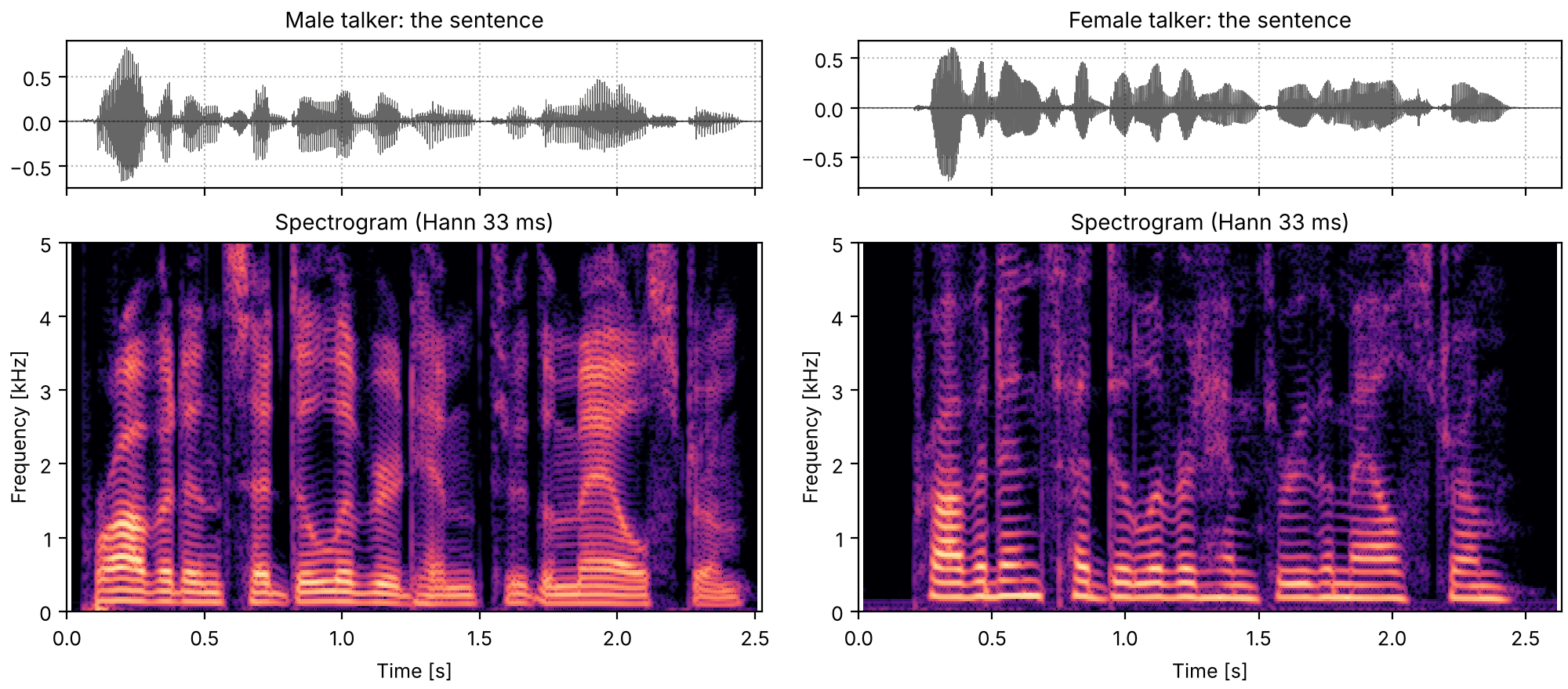
Plots of the the sentence, read by each talker sounds
Code
sounds = talkers
fig, playhead = show_pair(sounds, "the sentence")
Pitch

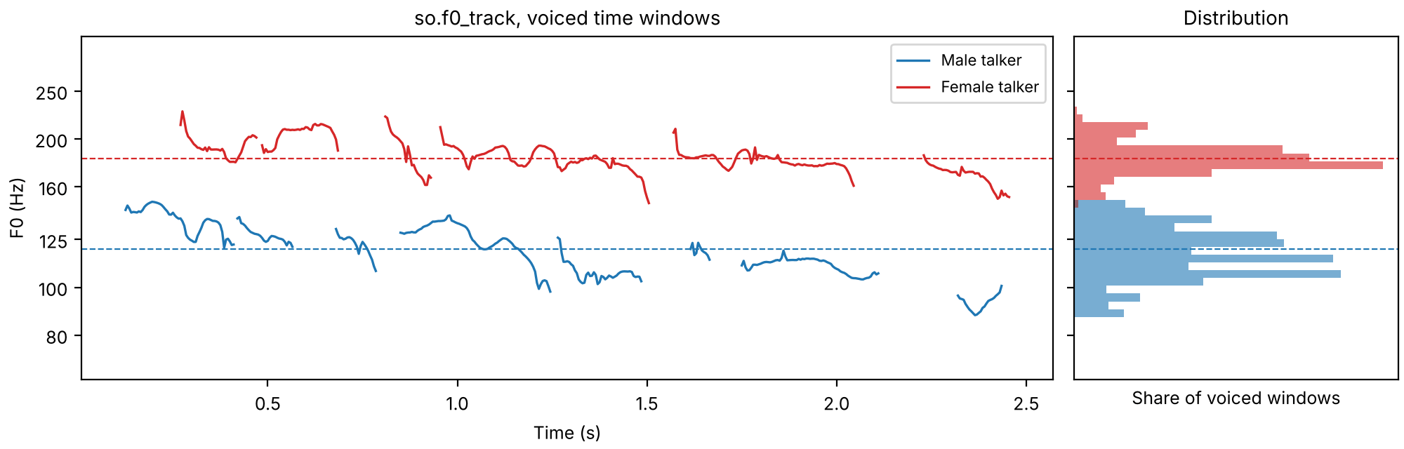
The median of the pitch track over its voiced time windows, and the range that holds the middle 90% of them. A ratio of pitches is also given in semitones, twelve to the octave.

Code
voiced_f0 = {label: track.f0[0][track.voiced[0]] for label, track in tracks.items()}
for label, f0 in voiced_f0.items():
    low, middle, high = np.percentile(f0, [5, 50, 95])
    span = 12 * np.log2(high / low)
    print(f"{label}: median {middle:.0f} Hz, middle 90% {low:.0f} to {high:.0f} Hz ({span:.1f} semitones)")
ratio = np.median(voiced_f0["Female talker"]) / np.median(voiced_f0["Male talker"])
print(f"female / male median: {ratio:.2f}, {12 * np.log2(ratio):.1f} semitones")
Male talker: median 119 Hz, middle 90% 95 to 142 Hz (7.0 semitones)
Female talker: median 183 Hz, middle 90% 164 to 211 Hz (4.3 semitones)
female / male median: 1.53, 7.4 semitones

The female talker's voice is about half as high again as the male talker's: a ratio of 1.53, a little more than a fifth (seven semitones, 1.50), and well short of an octave.

The two pitch tracks

Both pitch tracks against time, on a logarithmic frequency axis, where equal intervals are equal distances, and the share of voiced time windows at each pitch. The dashed lines are the medians.

The two pitch tracks
Code
fig, (left, right) = plt.subplots(
    1, 2, figsize=(10, 3.2), layout="constrained", width_ratios=[3, 1], sharey=True
)
bins = np.geomspace(70, 300, 41)
for color, (label, track) in zip(("C0", "C3"), tracks.items(), strict=True):
    left.plot(track.t, np.where(track.voiced[0], track.f0[0], np.nan), color=color, lw=1.2, label=label)
    right.hist(voiced_f0[label], bins=bins, orientation="horizontal", color=color, alpha=0.6, density=True)
    for ax in (left, right):
        ax.axhline(np.median(voiced_f0[label]), color=color, ls="--", lw=0.8)
left.set(yscale="log", xlabel="Time (s)", ylabel="F0 (Hz)", title="so.f0_track, voiced time windows")
left.set_yticks([80, 100, 125, 160, 200, 250], ["80", "100", "125", "160", "200", "250"])
left.set_yticks([], minor=True)
left.legend(loc="upper right", fontsize=8)
right.set(xlabel="Share of voiced windows", title="Distribution")
right.set_xticks([])

Spectral envelopes

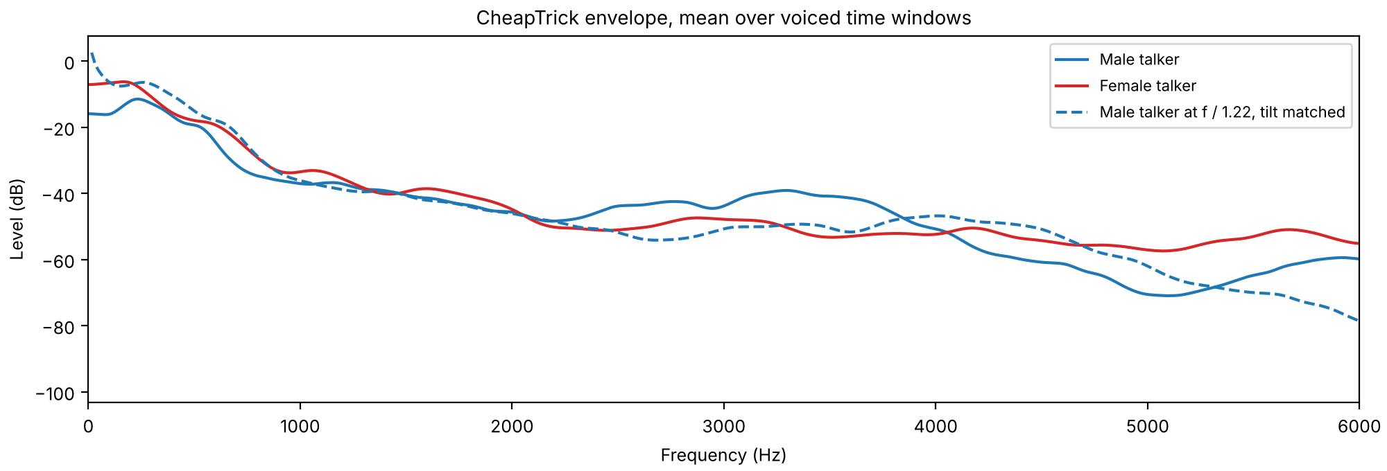
The formants are the peaks of the spectral envelope, the shape the vocal tract gives the harmonics. CheapTrick (Morise, 2015), which Spectral envelope explains, estimates it every 5 ms; averaging it in dB over each talker's voiced time windows gives one curve per talker. Shorter vocal tracts have higher formants, so a simple model of the difference reads the male envelope at f/r: every formant moved up by the same ratio r. The cell finds the r that brings the male average closest to the female one, with the overall level left free, and again with a tilt (a straight line in dB over log frequency) left free as well.

Code
envelopes = {label: so.cheaptrick(talkers[label], tracks[label]) for label in talkers}
frequencies = envelopes["Male talker"].f
scored = (frequencies >= 100) & (frequencies <= 5000)
average_db = {
    label: np.mean(10 * np.log10(env(tracks[label].t[tracks[label].voiced[0]], frequencies)[0]), axis=1)
    for label, env in envelopes.items()
}


def misfit(ratio, tilt=False):
    """RMS dB between the female average and the male one read at f / ratio, 100 to 5000 Hz,
    with the level (and, if tilt is True, a tilt) left free."""
    male_read = np.interp(frequencies[scored] / ratio, frequencies, average_db["Male talker"])
    difference = average_db["Female talker"][scored] - male_read
    columns = [np.ones(scored.sum())] + ([np.log2(frequencies[scored])] if tilt else [])
    basis = np.column_stack(columns)
    return np.sqrt(np.mean((difference - basis @ np.linalg.lstsq(basis, difference, rcond=None)[0]) ** 2))


ratios = np.arange(0.80, 1.60, 0.005)
for tilt in (False, True):
    errors = [misfit(r, tilt) for r in ratios]
    best = ratios[np.argmin(errors)]
    print(f"{'level and tilt free' if tilt else 'level free':20}: r = {best:.3f}, {min(errors):.2f} dB RMS")
warp = ratios[np.argmin([misfit(r, True) for r in ratios])]
level free          : r = 1.595, 4.52 dB RMS
level and tilt free : r = 1.220, 2.99 dB RMS

With only the level free, the best ratio is large, because the female talker's average envelope is also tilted differently, and moving formants is the only thing the fit can do about it. With the tilt free too, the ratio falls to 1.22. Changing a voice toward the other (Rebuilding and changing a voice) has to move the formants and the tilt separately.

The two average envelopes

The two average envelopes, and the male one read at f / r with the r just fitted with the tilt free, its level and tilt then matched to the female one over 100 to 5000 Hz.

The two average envelopes
Code
fig, ax = plt.subplots(figsize=(10, 3.4), layout="constrained")
male_read = np.interp(frequencies / warp, frequencies, average_db["Male talker"])
basis = np.column_stack([np.ones(scored.sum()), np.log2(frequencies[scored])])
level, tilt = np.linalg.lstsq(basis, average_db["Female talker"][scored] - male_read[scored], rcond=None)[0]
male_level = np.mean(average_db["Female talker"][scored] - average_db["Male talker"][scored])
ax.plot(frequencies, average_db["Male talker"] + male_level, color="C0", label="Male talker")
ax.plot(frequencies, average_db["Female talker"], color="C3", label="Female talker")
ax.plot(
    frequencies[1:],
    male_read[1:] + level + tilt * np.log2(frequencies[1:]),
    color="C0",
    ls="--",
    label=f"Male talker at f / {warp:.2f}, tilt matched",
)
ax.set(xlabel="Frequency (Hz)", ylabel="Level (dB)", xlim=(0, 6000))
ax.set_title("CheapTrick envelope, mean over voiced time windows")
ax.legend(loc="upper right", fontsize=8)

Long-term spectra

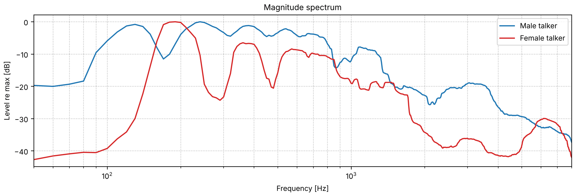
Averaged over the whole sentence, silences included, the spectrum shows where each reading puts its power (so.long_term_spectrum, as for the speech-shaped noise on Tones and noises). Averaged over many talkers, Byrne et al. (1994) found male and female long-term spectra nearly the same from 250 Hz to 5 kHz, with the male ones higher at 160 Hz and below, where their fundamentals lie. One sentence from each of two talkers can differ by more. The cell prints how each sentence's power divides among octave bands.

Code
spectra = {label: so.long_term_spectrum([snd]) for label, snd in talkers.items()}
octave_edges = [63, 125, 250, 500, 1000, 2000, 4000, 8000]
print("octave from [Hz]        " + "".join(f"{low:>6}" for low in octave_edges[:-1]))
for label, spectrum in spectra.items():
    power = 10 ** (spectrum.level / 10)
    shares = [
        10 * np.log10(power[(spectrum.f >= low) & (spectrum.f < high)].sum() / power.sum())
        for low, high in zip(octave_edges[:-1], octave_edges[1:], strict=True)
    ]
    print(f"{label + ', share [dB]':24}" + "".join(f"{share:6.1f}" for share in shares))
octave from [Hz]            63   125   250   500  1000  2000  4000
Male talker, share [dB]  -14.5  -8.5  -5.0  -4.7  -9.3 -14.3 -21.8
Female talker, share [dB] -41.1  -3.5  -7.9  -5.0 -12.6 -25.8 -18.6

Long-term spectra of the two talkers

The two long-term spectra, smoothed to a third of an octave. Below 125 Hz the female talker's sentence has almost nothing, since the female talker's pitch never goes that low, and the octave from 125 to 250 Hz, where it lies, holds most of the power. In this pair the female spectrum is also lower from 2 to 4 kHz and higher from 4 to 8 kHz.

Long-term spectra of the two talkers
Code
fig, ax = plt.subplots(figsize=(10, 3.4), layout="constrained")
for color, (label, spectrum) in zip(("C0", "C3"), spectra.items(), strict=True):
    spectrum.smooth(1 / 3).plot(ax, label=label, color=color)
ax.set_xlim(50, 8000)
ax.legend()
ax.grid(ls=":", which="both")

Harmonics sample the envelope

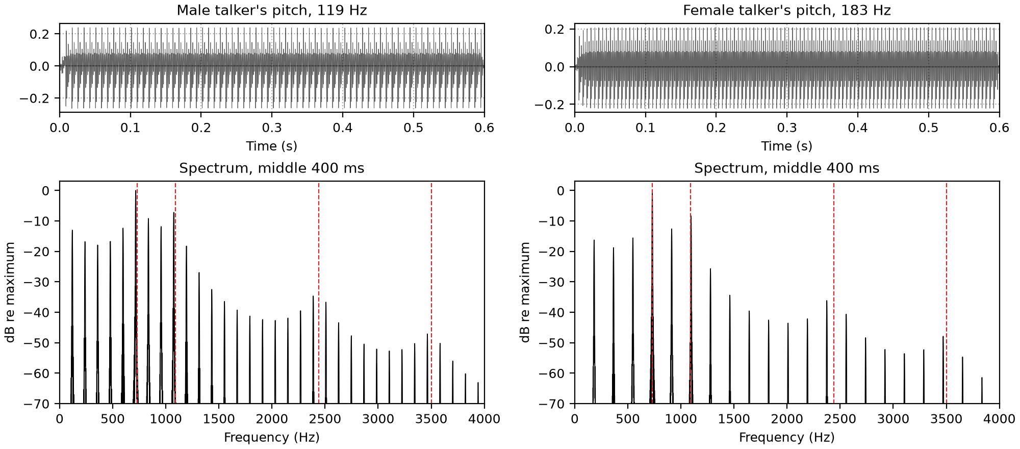
A voiced sound has energy only at the harmonics, multiples of F_0. The envelope, and with it the formants, is seen only where a harmonic falls: the harmonics sample it, once every F_0 hertz. To see that alone, the cell makes one vowel twice with so.klatt_synthesize (see Formant synthesis), with the same formants, those of a male "hod", at each talker's median pitch.

Code
FS = 16000
HOD = {"F1": 730, "F2": 1090, "F3": 2440, "F4": 3500, "F5": 4500}  # Peterson and Barney's male "hod"
medians = {label: float(np.median(f0)) for label, f0 in voiced_f0.items()}
vowels = {label: so.klatt_synthesize(0.6, FS, F0=f0, **HOD) for label, f0 in medians.items()}
for label, f0 in medians.items():
    print(f"{label}: F0 {f0:.0f} Hz, {int(1000 // f0)} harmonics below 1 kHz")
Male talker: F0 119 Hz, 8 harmonics below 1 kHz
Female talker: F0 183 Hz, 5 harmonics below 1 kHz

One vowel at the two pitches

The vowel at each pitch: the same formants, and so the same vowel, sampled by harmonics at different spacings. Left, the spectrum of the middle 400 ms, with the five formants dashed. The female talker's pitch puts fewer harmonics under each formant peak, so the peaks are drawn by fewer points, and a harmonic can miss a peak by up to half the spacing.

Male talker

tk5_one_vowel_at_the_two_pitches_male_talker.flac, 0.6 s, mono

Female talker

tk5_one_vowel_at_the_two_pitches_female_talker.flac, 0.6 s, mono

Plots of the one vowel at the two pitches sounds
Code
sounds = {label: finish(v) for label, v in vowels.items()}
fig = plt.figure(figsize=(10, 4.4), layout="constrained")
columns = fig.subfigures(1, 2)
playhead = {}
for column, (label, snd) in zip(columns, sounds.items(), strict=True):
    top, bottom = column.subplots(2, 1, height_ratios=[0.4, 1])
    snd.plot(top, color="k", lw=0.4)
    top.set(
        title=f"{label}'s pitch, {medians[label]:.0f} Hz",
        xlabel="Time (s)",
        ylabel="",
        xlim=(0, snd.duration),
    )
    middle = snd.data[int(0.1 * FS) : int(0.5 * FS), 0] * np.hanning(int(0.4 * FS))
    spectrum = 20 * np.log10(np.abs(np.fft.rfft(middle, 8 * len(middle))) + 1e-9)
    bottom.plot(np.fft.rfftfreq(8 * len(middle), 1 / FS), spectrum - spectrum.max(), color="k", lw=0.6)
    for f in HOD.values():
        bottom.axvline(f, color="C3", ls="--", lw=0.8)
    bottom.set(xlim=(0, 4000), ylim=(-70, 3), xlabel="Frequency (Hz)", ylabel="dB re maximum")
    bottom.set_title("Spectrum, middle 400 ms")
    playhead[label] = [top]

The same sampling sets limits on every page that follows, a little tighter for the female talker:

  • Seeing speech: harmonics farther apart are easier to resolve, and a narrowband spectrogram can use a shorter window.
  • Pitch tracking: a window of fixed length holds more periods of the higher voice, but the cepstrum's second peak, at two periods, then falls inside the range searched for the pitch, and can be taken for it.
  • Spectral envelope: the envelope has to be read between fewer samples, so a cepstral lifter has to cut lower and CheapTrick's error grows.
  • Source and aperiodicity: fewer harmonics are left to measure the noise between.
  • Formant synthesis: the female vowels, made with female formants.

References

  • Byrne et al. (1994). An international comparison of long-term average speech spectra. JASA 96(4), 2108–2120. doi:10.1121/1.410152.
  • Kominek & Black (2004). The CMU Arctic speech databases. Proc. 5th ISCA Speech Synthesis Workshop, 223–224. ISCA Archive. The sentence, by speakers bdl and slt.
  • Morise (2015). CheapTrick, a spectral envelope estimator for high-quality speech synthesis. Speech Communication 67. doi:10.1016/j.specom.2014.09.003.
  • Peterson & Barney (1952). Control methods used in a study of the vowels. JASA 24(2), 175–184. doi:10.1121/1.1906875.