Streams: reproducing Bregman & Ahad

Every sound on this page is sonore's reproduction of a published demonstration. Almost all of them are from Albert Bregman and Pierre Ahad's Demonstrations of Auditory Scene Analysis (1996), a compact disc made to accompany Bregman's book Auditory Scene Analysis (1990); one is from the Acoustical Society of America's Auditory Demonstrations (Houtsma, Rossing & Wagenaars, 1987). The demonstrations, their design and what they show are their authors' work. Bregman's laboratory publishes the original recordings and booklet (McGill), and they are the ones to listen to.

What they show. When sounds follow one another, hearing sorts them into streams: sequences heard as coming from one source, like one voice or one instrument. Sounds close in pitch, timbre or location tend to join one stream; sounds far apart, played fast, split into separate streams, and you hear two things at once. Once a sequence has split, what lies across the streams gets hard to hear: which tone came before which, or the rhythm the tones make together. Bregman called this auditory stream segregation. Each section below varies one thing that makes a sequence split or hold together, and each example opens with what to listen for, taken from what its booklet reports listeners hear.

This page is a test of sonore: can its generators rebuild each stimulus from the description in the booklet? Each example names the demonstration it reproduces, rebuilds it from the booklet's frequencies, levels and timing, and says where it departs from them: where the booklet leaves a value open, where a recording is replaced by a stand-in, or where a long track is shortened. What listeners hear is reported as the booklet reports it; this page has not tested any of it.

  • Speed and frequency: a six-tone cycle that splits into two melodies when played fast, and a gallop that loses its rhythm (Bregman & Ahad, Demonstrations 1–3; Houtsma et al., Demonstration 19).
  • Streaming builds up: the same gallop in runs of 2 to 32 (Demonstration 4).
  • A hidden melody: a tune interleaved with distractors, moved away from them (Demonstration 5).
  • Timbre and spectrum: tones of one pitch split by where their spectrum peaks, vowels, and bands of noise (Demonstrations 10, 11 and 14).
  • Glides and timing: glides that hold a sequence together, and timing that is hard to judge across streams (Demonstrations 12 and 13).
  • Competition and capture: which tones group depends on the others present (Demonstrations 15–17).
  • Interlocking parts: two interleaved parts split by pitch, timbre and place, with a stand-in for the East African xylophone music on the disc (Demonstrations 7–9 and 41).
  • Place: noise bursts that split when they come from two sides (Demonstrations 38 and 39).

Headphones are best for the last two sections, which send different sounds to the two ears.

Setup, the same on every page
import os
import urllib.request

import matplotlib.pyplot as plt
import numpy as np

import sonore as so

plt.rcParams.update({"font.size": 9, "axes.titlesize": 10, "figure.dpi": 100})


def fetch(path):
    """A file from the sonore repository, by its path there: the local copy when this runs from
    the repository root, otherwise downloaded from GitHub to the same relative path."""
    if not os.path.exists(path):
        os.makedirs(os.path.dirname(path) or ".", exist_ok=True)
        urllib.request.urlretrieve("https://raw.githubusercontent.com/choyun1/sonore/main/" + path, path)
    return path


def finish(snd):
    """How every sound in the gallery is played: 5 ms ramps, RMS 0.1, peak at most 0.95."""
    snd = snd.ramp(5e-3).normalize(rms=0.1)
    return snd.normalize(peak=0.95) if snd.peak > 0.95 else snd

Press play and a line follows the sound across every time axis in its plots. Click any time axis to play from that point. The audio is lossless, since compression would alter the binaural sounds. Start with your volume low.

To run this page yourself, open it as a notebook in Colab or download it. It is the same code, and it fetches the recordings it needs from the sonore repository.

Code the examples share

Every sound is built from timed events: a tone or a noise burst, placed at its onset time. The booklet gives levels relative to the other sounds in a demonstration, and finish keeps those relations, scaling only the whole sound. The sample rate is 22.05 kHz, enough for everything on the page, which has nothing above 4 kHz except the white noise of the last section.

Code
FS = 22050


def tone(freq, dur, rise=10e-3, decay=10e-3, db=0.0):
    """A sine tone `dur` seconds long including linear rise and decay ramps, `db` re the others."""
    n = round(dur * FS)
    env = np.minimum(1, np.minimum(np.arange(n) / (rise * FS), np.arange(n)[::-1] / (decay * FS)))
    return so.Sound(env * so.pure_tone(dur, FS, freq).data[:, 0], FS).gain_db(db)


def place(events, dur=None):
    """Sounds added at their onset times: `events` is a list of (onset in seconds, Sound)."""
    end = max(onset + snd.duration for onset, snd in events)
    n_channels = max(snd.n_channels for _, snd in events)
    out = np.zeros((round((dur or end) * FS) + 1, n_channels))
    for onset, snd in events:
        i = round(onset * FS)
        out[i : i + snd.n_samples] += snd.data[: len(out) - i]
    return so.Sound(out, FS)


def gallop(high, low, onsets):
    """HLH- triplets: `onsets` is every unit's onset; a unit is a tone or the silence after a triplet."""
    return [(t, (high, low, high, None)[i % 4]) for i, t in enumerate(onsets) if i % 4 != 3]


def accelerating(n_units, first, last):
    """Onsets of `n_units` units whose length shrinks geometrically from `first` to `last` seconds."""
    lengths = np.geomspace(first, last, n_units)
    return np.concatenate([[0], np.cumsum(lengths[:-1])]), lengths


def show(snd, fmin=100, fmax=5000, title="Spectrogram (Hann 30 ms)"):
    """A spectrogram on a log frequency axis, one panel per channel. Returns the figure and the
    panels the playhead follows."""
    n = snd.n_channels
    fig, axes = plt.subplots(
        n, 1, figsize=(10, 2.6 + 1.6 * n), sharex=True, layout="constrained", squeeze=False
    )
    stft = so.STFT(snd, win_dur=30e-3, hop_dur=5e-3)
    keep = (stft.f >= fmin) & (stft.f <= fmax)
    top = stft.db[:, keep].max()
    for ch, ax in enumerate(axes[:, 0]):
        ax.pcolormesh(stft.t, stft.f[keep], stft.db[ch][keep], vmin=top - 60, vmax=top, cmap="magma")
        side = f", {('left', 'right')[ch]} ear" if n == 2 else ""
        so.plotting.log_frequency_axis(ax)
        ax.set(ylim=(fmin, fmax), ylabel="Frequency [Hz]", title=title + side)
    axes[-1, 0].set(xlabel="Time [s]", xlim=(0, snd.duration))
    return fig, list(axes[:, 0])

Speed and frequency

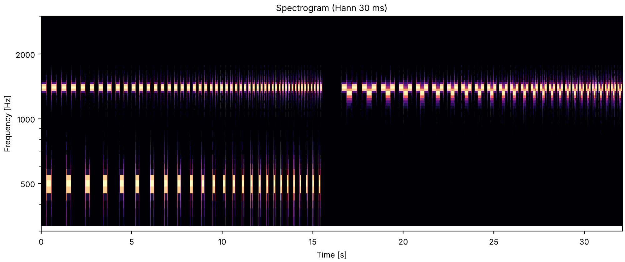
Bregman & Ahad's first demonstration, after an experiment by Bregman & Campbell (1971), is a repeating cycle of three high and three low tones in strict alternation. Their booklet reports that played slowly it is heard as one six-note melody, and played fast it splits into a high and a low stream, each with its own three-note melody, so that the order of high and low tones becomes hard to report.

A six-tone cycle, slow then fast

Listen for the slow cycle as one six-note tune, and the fast one splitting into two three-note tunes, one high and one low, heard at once. Try to say which low tone follows which high one.

Bregman & Ahad, Demonstration 1. Highs of 2500, 2000 and 1600 Hz alternate with lows of 350, 430 and 550 Hz in the order H1 L1 H2 L2 H3 L3, with no silences and 10 ms onsets and offsets, the lows 6 dB stronger, as in the booklet: three cycles with 400 ms from one onset to the next, then, after a second's silence, twelve cycles at 100 ms. The booklet gives no repetition counts; these are ours.

sg1_a_six-tone_cycle_slow_then_fast.flac, 15.4 s, mono
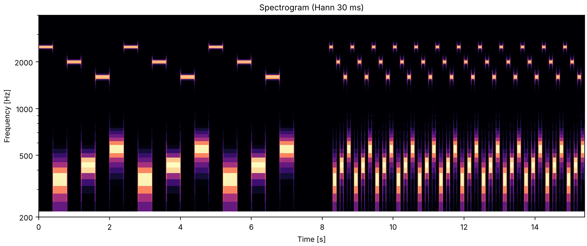
Plots of the a six-tone cycle, slow then fast sound
Code
HIGHS, LOWS = (2500, 2000, 1600), (350, 430, 550)


def six_tone_cycle(period, n_cycles, start=0.0, low_db=6.0):
    pairs = zip(HIGHS, LOWS, strict=True)
    cycle = [tone(f, period, db=low_db * (i % 2)) for pair in pairs for i, f in enumerate(pair)]
    return [(start + period * (6 * c + k), cycle[k]) for c in range(n_cycles) for k in range(6)]


sound = finish(place(six_tone_cycle(0.4, 3) + six_tone_cycle(0.1, 12, start=8.2)))
fig, playhead = show(sound, fmin=200, fmax=4000)
Standards within and across streams

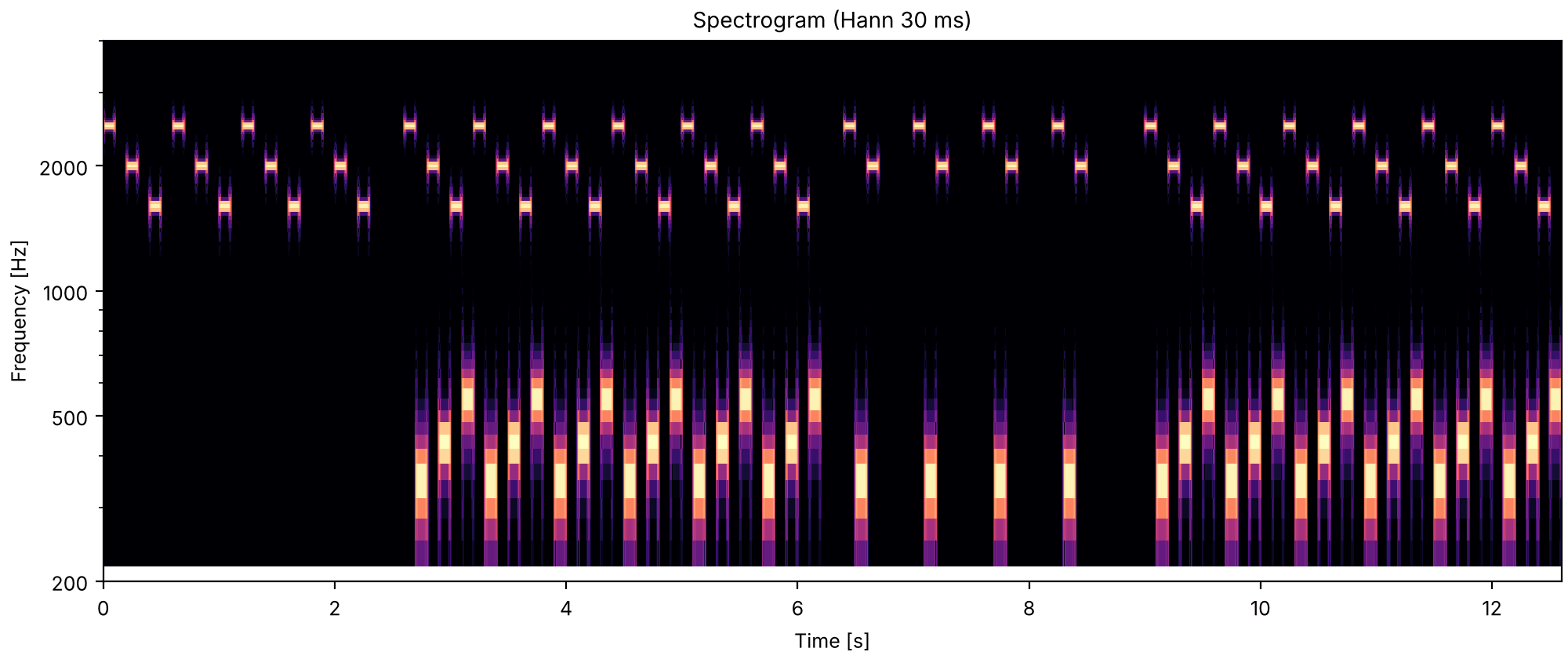
Listen for the three-tone standard inside the fast cycle. The first standard, all high tones, should be easy to find; the second, high, low, high, very hard.

Bregman & Ahad, Demonstration 2. A three-tone standard, the fast cycle with three of its tones replaced by silence, is heard first, then the full cycle, in which a listener tries to keep hearing the standard. The booklet's lows are 1.5 dB stronger here. First a standard of the three highs, which lie in one stream, then a standard of two highs and the low between them (H1 L1 H2), which crosses streams; the booklet reports the first easy to hear in the cycle and the second very hard. The booklet makes its across-stream standard evenly spaced in time by changing the full pattern; this reproduction keeps the strict alternation, so its across-stream standard is not evenly spaced.

sg2_standards_within_and_across_streams.flac, 12.6 s, mono

Plots of the standards within and across streams sound
Code
def standard(keep, n_cycles, start):
    events = six_tone_cycle(0.1, n_cycles, start, low_db=1.5)
    return [event for i, event in enumerate(events) if i % 6 in keep]


events = []
for start, keep in ((0.0, {0, 2, 4}), (6.4, {0, 1, 2})):
    events += standard(keep, 4, start) + six_tone_cycle(0.1, 6, start + 2.6, low_db=1.5)
sound = finish(place(events))
fig, playhead = show(sound, fmin=200, fmax=4000)
A gallop that speeds up

Listen for the first gallop's da-da-dum rhythm breaking apart as it speeds up, into a fast high beat and a slow low one. The second gallop, its tones close in pitch, keeps galloping.

Bregman & Ahad, Demonstration 3, after van Noorden (1975). Triplets HLH, each followed by a silence as long as a tone, speeding up from 287 to 88 ms per unit (a tone or the silence); the tones fill their units, with 10 ms rises and 20 ms decays. First with H and L 17.8 semitones apart (1400 and 500 Hz), then one semitone apart (1400 and 1320 Hz). The booklet reports that the first loses its galloping rhythm as it speeds up, splitting into a fast high stream and a slow low one, and that the second keeps galloping. How quickly the gallop speeds up is not in the booklet; here it takes 20 triplets and then holds the fastest speed for 6.

sg3_a_gallop_that_speeds_up.flac, 32.1 s, mono

Plots of the a gallop that speeds up sound
Code
def speeding_gallop(high_hz, low_hz, start):
    onsets, lengths = accelerating(4 * 20, 0.287, 0.088)
    onsets = np.concatenate([onsets, onsets[-1] + 0.088 * np.arange(1, 4 * 6 + 1)])
    lengths = np.concatenate([lengths, np.full(4 * 6, 0.088)])
    events = []
    for i, (t, length) in enumerate(zip(onsets, lengths, strict=True)):
        if i % 4 != 3:
            events.append((start + t, tone((high_hz, low_hz, high_hz)[i % 4], length, decay=20e-3)))
    return events, start + onsets[-1] + 0.088


first, end = speeding_gallop(1400, 500, 0.0)
second, _ = speeding_gallop(1400, 1320, end + 1.0)
sound = finish(place(first + second))
fig, playhead = show(sound, fmin=300, fmax=3000)

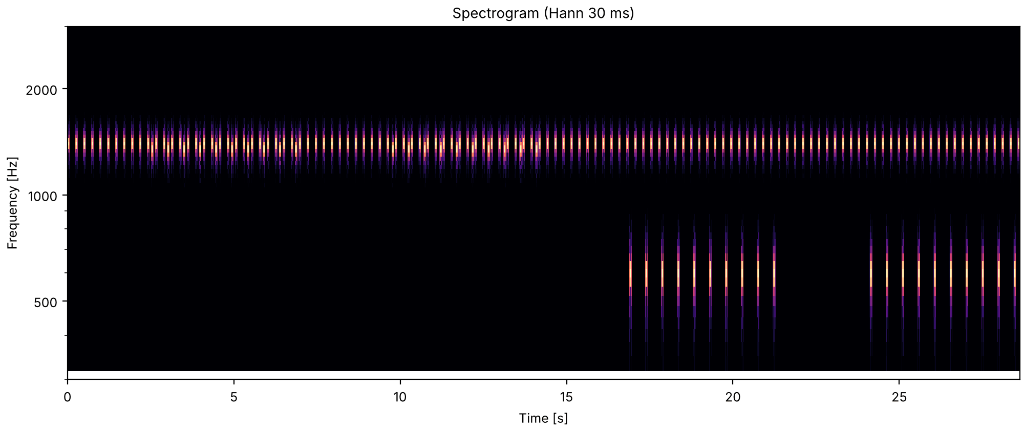
B sweeps past A

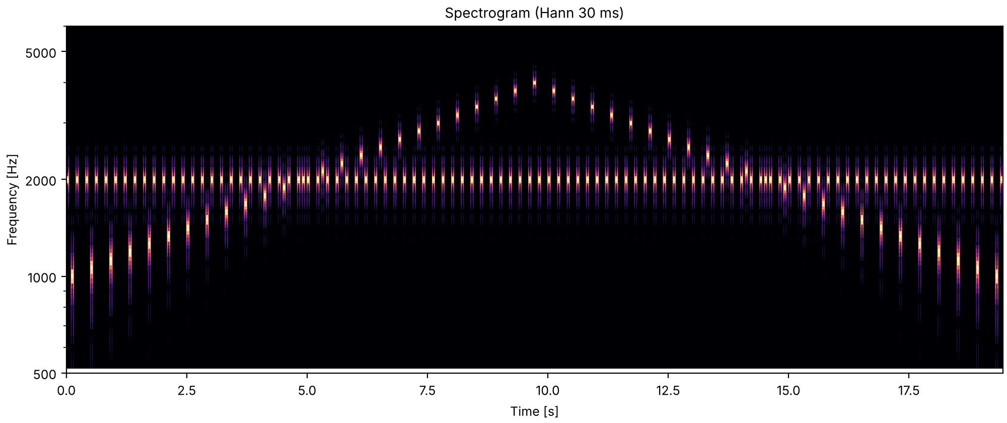
Listen for a gallop while B is near A in pitch, in the middle of the sound, and two separate, evenly beating sequences while B is far above or below.

Houtsma, Rossing & Wagenaars, Demonstration 19, after van Noorden (1975), whose thesis introduced the gallop. Tone A stays at 2000 Hz; tone B steps from 1000 Hz up to 4000 Hz and back, in the ABA- rhythm. Their booklet reports a galloping rhythm near the crossing and two separate sequences when A and B are far apart. It gives neither the tone length nor the rate; here the tones are 50 ms with 5 ms ramps, 100 ms apart, and B moves one semitone per triplet.

sg4_b_sweeps_past_a.flac, 19.5 s, mono

Plots of the b sweeps past a sound
Code
steps = np.concatenate([np.arange(0, 24), np.arange(24, -1, -1)])
events = []
for k, semitones in enumerate(steps):
    b = tone(1000 * 2 ** (semitones / 12), 0.05, 5e-3, 5e-3)
    a = tone(2000, 0.05, 5e-3, 5e-3)
    events += [(0.4 * k, a), (0.4 * k + 0.1, b), (0.4 * k + 0.2, a)]
sound = finish(place(events))
fig, playhead = show(sound, fmin=500, fmax=6000)

Streaming builds up

Splitting takes time: a sequence often starts as one stream and splits after a few seconds of listening.

Runs of 2 to 32 gallops

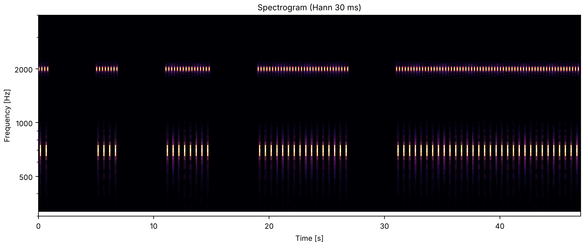
Listen for the gallop holding together in the short runs and splitting into a high and a low beat during the long ones.

Bregman & Ahad, Demonstration 4. The gallop of a 2000 Hz H and a 700 Hz L, each tone a 12.5 ms rise, 88 ms steady and 12.5 ms decay then 12 ms of silence (125 ms a unit), the low tone 6 dB stronger, in runs of 2, 4, 8, 16 and 32 triplets separated by 4 s of silence, all as in the booklet. Its reasoning: if a tendency to split builds up while the gallop plays and dies away in silence, the longer runs should split more. This is the page's longest sound, 47 s, because the build-up is the point.

sg5_runs_of_2_to_32_gallops.flac, 47.0 s, mono

Plots of the runs of 2 to 32 gallops sound
Code
h, l = tone(2000, 0.113, 12.5e-3, 12.5e-3), tone(700, 0.113, 12.5e-3, 12.5e-3, db=6)
events, start = [], 0.0
for run in (2, 4, 8, 16, 32):
    events += [(start + t, snd) for t, snd in gallop(h, l, 0.125 * np.arange(4 * run))]
    start += 0.5 * run + 4.0
sound = finish(place(events, dur=start - 4.0))
fig, playhead = show(sound, fmin=300, fmax=4000)

A hidden melody

Splitting can hide a tune among other notes, or free it.

A melody pulling away from its distractors

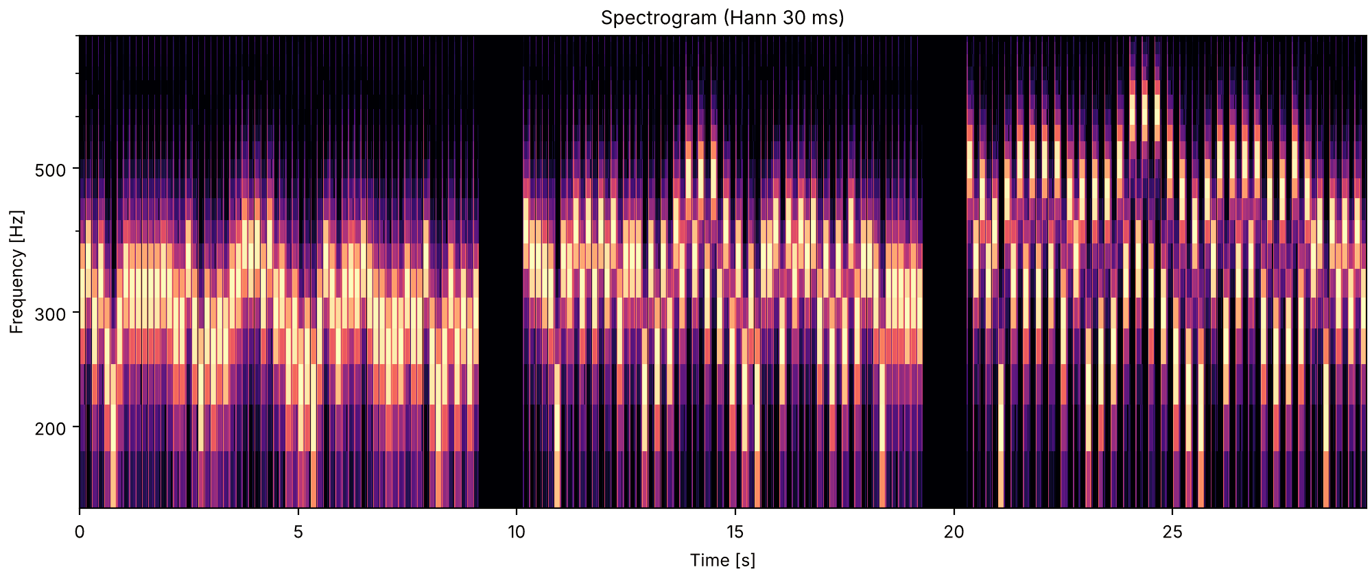
Listen for a familiar tune hidden among the notes. In the first presentation it is lost among the distractors; by the last it stands out above them.

Bregman & Ahad, Demonstration 5, after Dowling (1973). A familiar tune's notes, each long note broken into quarter notes, alternate with random distractors, 7 tones a second (3 ms rise, 97 ms steady, 20 ms decay, 23 ms silence). The melody starts between C4 and G4, with C4 at 256 Hz as in the booklet, and moves up four semitones on each of three presentations (the booklet has five presentations, two semitones apart, ending at the same place); each distractor is drawn within four semitones of the previous note of the untransposed melody, so the distractors stay where they were. The booklet reports the tune hidden at first and easier to hear as it pulls away. The booklet keeps the tune secret until its last page; the code below names it. The tune and the seed of the distractors are ours to choose, as the booklet's choices are only partly given.

sg6_a_melody_pulling_away_from_its_distractors.flac, 29.4 s, mono

Plots of the a melody pulling away from its distractors sound
Code
# Mary Had a Little Lamb, in semitones above C4, long notes broken into quarter notes.
melody = [4, 2, 0, 2, 4, 4, 4, 4, 2, 2, 2, 2, 4, 7, 7, 7, 4, 2, 0, 2, 4, 4, 4, 4, 2, 2, 4, 2, 0, 0, 0, 0]
rng = np.random.default_rng(5)
distractors = [m + rng.integers(-4, 5) for m in melody]
events, t = [], 0.0
for shift in (0, 4, 8):
    for note, other in zip(melody, distractors, strict=True):
        for semitones in (note + shift, other):
            events.append((t, tone(256 * 2 ** (semitones / 12), 0.12, rise=3e-3, decay=20e-3)))
            t += 0.143
    t += 1.0
sound = finish(place(events))
fig, playhead = show(sound, fmin=150, fmax=800)

Timbre and spectrum

Streams also split by timbre, with the pitch held fixed.

One pitch, two spectral peaks

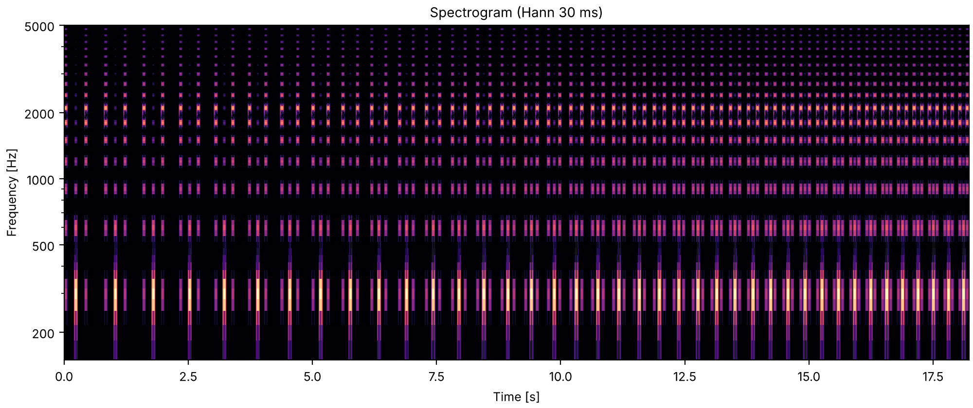
Listen for tones of one pitch splitting into a bright stream and a dull one as the gallop speeds up.

Bregman & Ahad, Demonstration 10. Two tones on the same 300 Hz fundamental, 30 equal harmonics through a resonance 80 Hz wide, peaking at 2000 Hz (H, bright) or 300 Hz (L, dull), 65 ms long with 20 ms rises and decays, the dull ones 3 dB stronger at their peaks. They gallop, HLH- with a 65 ms silence for the missing L, and the silences between sounds shrink from 140 to 10 ms (from about 5 to 13 tones a second). The booklet reports the bright and dull tones separating as the gallop speeds up. sonore's so.resonator is Klatt's second-order resonator; the booklet does not name its formant filter, and the number of triplets (40 here) is ours.

sg7_one_pitch_two_spectral_peaks.flac, 18.2 s, mono

Plots of the one pitch, two spectral peaks sound
Code
def peaked(center):
    buzz = so.harmonic_complex(0.065, FS, 300, harmonics=np.arange(1, 31), phases="sine")
    snd = so.resonator(buzz, center, 80)
    n = snd.n_samples
    ramp = np.minimum(1, np.minimum(np.arange(n), np.arange(n)[::-1]) / (20e-3 * FS))
    return so.Sound(ramp * snd.data[:, 0] / np.abs(snd.data).max(), FS)


bright, dull = peaked(2000), peaked(300).gain_db(3)
silences = np.geomspace(0.140, 0.010, 4 * 40)
onsets = np.concatenate([[0], np.cumsum(0.065 + silences[:-1])])
sound = finish(place(gallop(bright, dull, onsets)))
fig, playhead = show(sound, fmin=150, fmax=5000)

Vowels in alternation

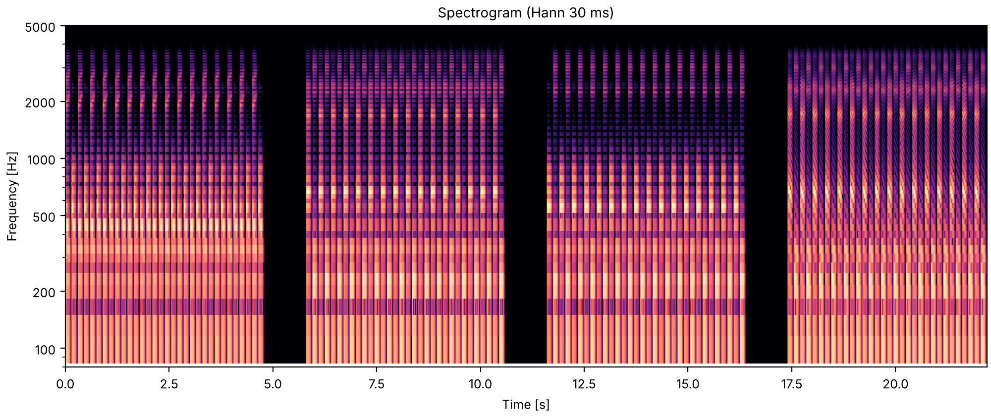
Listen for the alternating vowels splitting into two streams, each repeating one vowel.

Bregman & Ahad, Demonstration 11. Short vowels alternating: "ay" (as in hay) with "o" (hoe), "a" (had) with "ee" (he), and "aw" (haw) with "ee", at a steady 112 Hz, then "a" with "ee" on a pitch falling from 118 to 92 Hz. The booklet used Peterson & Barney's (1952) formant frequencies and an envelope of a 20 ms rise, an 80 ms decline and an exponential decay (10 ms time constant). It reports that the vowels split into streams, with or without the pitch movement. Here they come from so.klatt_synthesize, with Peterson & Barney's averages for men; the two diphthongs glide between two of their vowels (our choice, since they measured no diphthongs), each vowel lasts 150 ms, the decline falls to half amplitude, and there are 16 alternations of each pair instead of the booklet's 32.

sg8_vowels_in_alternation.flac, 22.2 s, mono

Plots of the vowels in alternation sound
Code
VOWELS = {  # F1, F2, F3 [Hz], Peterson & Barney (1952), men
    "ee": (270, 2290, 3010), "eh": (530, 1840, 2480), "a": (660, 1720, 2410),
    "aw": (570, 840, 2410), "oo": (300, 870, 2240),
}
DIPHTHONGS = {"ay": ("eh", "ee"), "o": ("aw", "oo")}


def vowel(name, f0):
    start, end = (VOWELS[v] for v in DIPHTHONGS.get(name, (name, name)))
    times = np.array([0.0, 0.15])
    tracks = {f"F{k + 1}": (times, [start[k], end[k]]) for k in range(3)}
    snd = so.klatt_synthesize(0.15, FS, F0=(times, f0), **tracks)
    t = snd.t
    decay = np.where(t < 0.1, 1 - 0.5 * (t - 0.02) / 0.08, 0.5 * np.exp(-(t - 0.1) / 0.01))
    env = np.where(t < 0.02, t / 0.02, decay)
    return so.Sound(env * snd.data[:, 0], FS).normalize(rms=0.1)


events, t = [], 0.0
pairs = [(("ay", "o"), [112, 112]), (("a", "ee"), [112, 112]), (("aw", "ee"), [112, 112])]
for pair, f0 in pairs + [(("a", "ee"), [118, 92])]:
    two_vowels = [vowel(name, f0) for name in pair]
    for k in range(32):
        events.append((t, two_vowels[k % 2]))
        t += 0.15
    t += 1.0
sound = finish(place(events))
fig, playhead = show(sound, fmin=80, fmax=5000)

High and low bands of noise

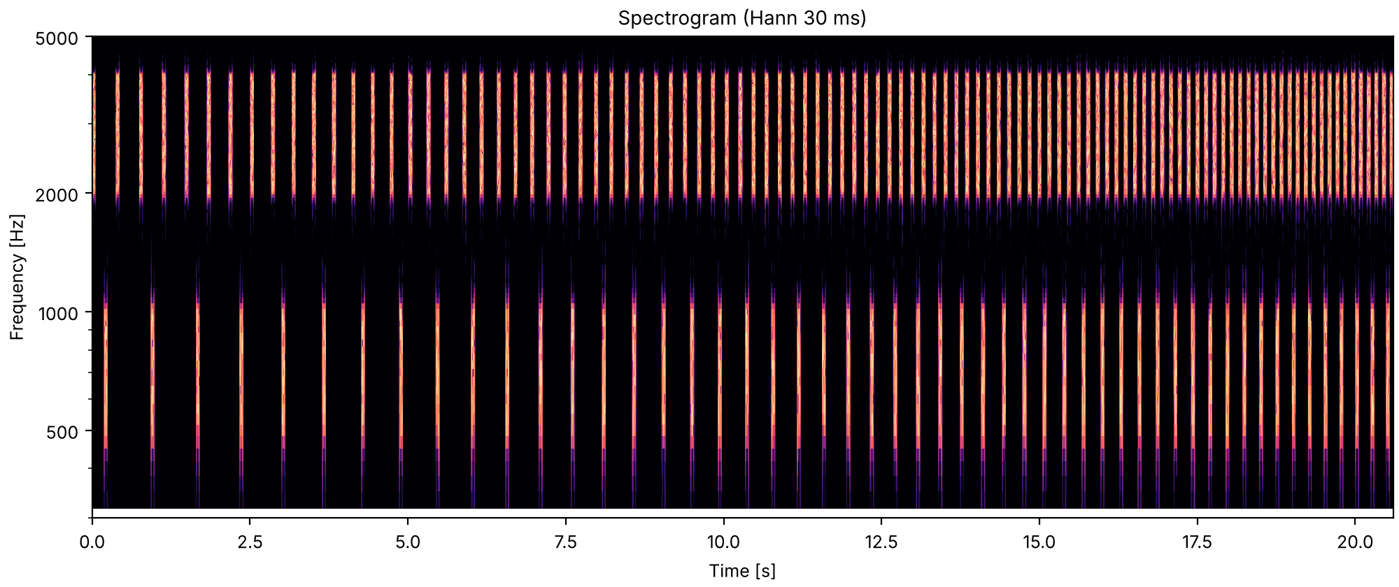
Listen for the noise gallop splitting into a high hiss and a low hiss as it speeds up, as tones do.

Bregman & Ahad, Demonstration 14, after Dannenbring & Bregman (1976). Noise bursts in a gallop: a low band from 500 to 1000 Hz and a high band from 2000 to 4000 Hz, 50 ms long with 5 ms rises and decays. As in the booklet, each burst is a sum of equal tones in random phase, 2 Hz apart in the low band and 3 Hz in the high one, which gives flat bands with sharp edges, at equal spectrum level; the silences between elements (a burst, or the 50 ms gap after a triplet) shrink from 140 to 10 ms over 52 triplets. The booklet reports that the bands split as tones do.

sg9_high_and_low_bands_of_noise.flac, 20.6 s, mono

Plots of the high and low bands of noise sound
Code
rng = np.random.default_rng(14)


def band(lo, hi, step):
    """Equal tones `step` Hz apart in random phase from `lo` to `hi`, at a spectrum level that
    does not depend on `step`: a burst of noise with sharp edges."""
    harmonics = np.arange(round(lo / step), round(hi / step) + 1)
    phases = rng.uniform(0, 2 * np.pi, len(harmonics))
    snd = so.harmonic_complex(0.05, FS, step, harmonics=harmonics, phases=phases, ramp=0)
    # It comes out at RMS 1, as every sonore generator's sound does; scaled so that each tone has
    # power `step`, the band has power 1 per Hz.
    snd = snd * np.sqrt(len(harmonics) * step)
    n = snd.n_samples
    ramp = np.minimum(1, np.minimum(np.arange(n), np.arange(n)[::-1]) / (5e-3 * FS))
    return so.Sound(ramp * snd.data[:, 0], FS)


silences = np.geomspace(0.140, 0.010, 4 * 52)
onsets = np.concatenate([[0], np.cumsum(0.05 + silences[:-1])])
high_band, low_band = (2000, 4000, 3), (500, 1000, 2)
events = [(t, band(*(low_band if i % 4 == 1 else high_band))) for i, t in enumerate(onsets) if i % 4 != 3]
sound = finish(place(events))
fig, playhead = show(sound, fmin=300, fmax=5000)

Glides and timing

A smooth path from tone to tone holds a sequence together, and timing is hard to judge across two streams.

Tones joined by glides, then not

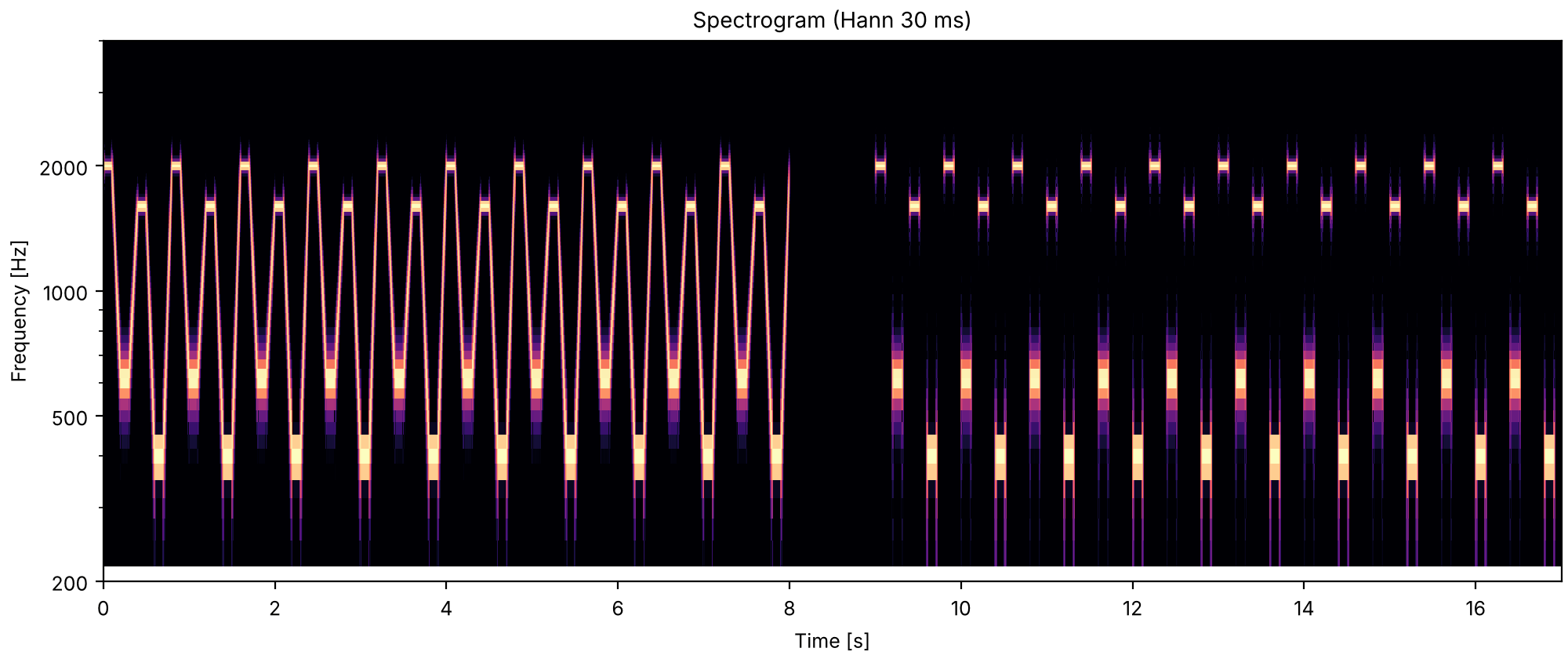
Listen for the joined version as one wavy line, and the tones without glides splitting into high and low streams sooner.

Bregman & Ahad, Demonstration 12, after Bregman & Dannenbring (1973). The cycle 2000, 614, 1600, 400 Hz, ten times (the booklet plays it twenty), first with each tone joined to the next by a glide (100 ms steady, 100 ms gliding, straight on a log-frequency axis), then with the glides left out: 100 ms tones with 10 ms rises and decays and the rest of each 200 ms slot silent. The booklet reports the joined sequence heard as more coherent, and streaming building up faster without the glides.

sg10_tones_joined_by_glides_then_not.flac, 17.0 s, mono

Plots of the tones joined by glides, then not sound
Code
FREQS = [2000, 614, 1600, 400]
times = np.linspace(0, 8, 8 * 400 + 1)
slot, within = np.divmod(times, 0.2)
f_from = np.take(FREQS, slot.astype(int) % 4)
f_to = np.take(FREQS, (slot.astype(int) + 1) % 4)
glide = np.clip((within - 0.1) / 0.1, 0, 1)
contour = f_from * (f_to / f_from) ** glide
joined = so.harmonic_complex(8, FS, (times, contour), harmonics=[1], ramp=0)
apart = place([(0.2 * k, tone(FREQS[k % 4], 0.12)) for k in range(40)], dur=8)
sound = finish(so.concat([joined.ramp(0.01), so.silence(1.0, FS), apart]))
fig, playhead = show(sound, fmin=200, fmax=4000)
Where the low tone falls

Listen for the low tone sitting off center in the gap. It should be easy to hear when it is close in pitch to the repeating tone (the first two sets) and hard when it is far below (the last two).

Bregman & Ahad, Demonstration 13, after van Noorden (1975). A 1400 Hz tone H repeats throughout: 60 ms tones (20 ms rises and decays) with 180 ms between them. Four times a low tone L is brought in for ten ABA triplets, in every other gap: at 1350 Hz centered in the gap, at 1350 Hz 30 ms late (90 ms before it, 30 after), at 600 Hz 30 ms early, and at 600 Hz centered. The booklet reports the off-center L easy to hear at 1350 Hz, in the same stream as H, and hard at 600 Hz, in a stream of its own. How long H plays alone between the sets (five triplets here) is ours.

sg11_where_the_low_tone_falls.flac, 28.6 s, mono

Plots of the where the low tone falls sound
Code
h = tone(1400, 0.06, 20e-3, 20e-3)
events, t = [], 0.0
for low_hz, offset in [(1350, 0.0), (1350, 0.03), (600, -0.03), (600, 0.0)]:
    l_tone = tone(low_hz, 0.06, 20e-3, 20e-3)
    for k in range(15):
        events += [(t, h), (t + 0.24, h)]
        if k >= 5:
            events.append((t + 0.06 + 0.06 + offset, l_tone))
        t += 0.48
sound = finish(place(events))
fig, playhead = show(sound, fmin=300, fmax=3000)

Competition and capture

Whether two tones fall in one stream depends not only on how far apart they are but on what else is playing.

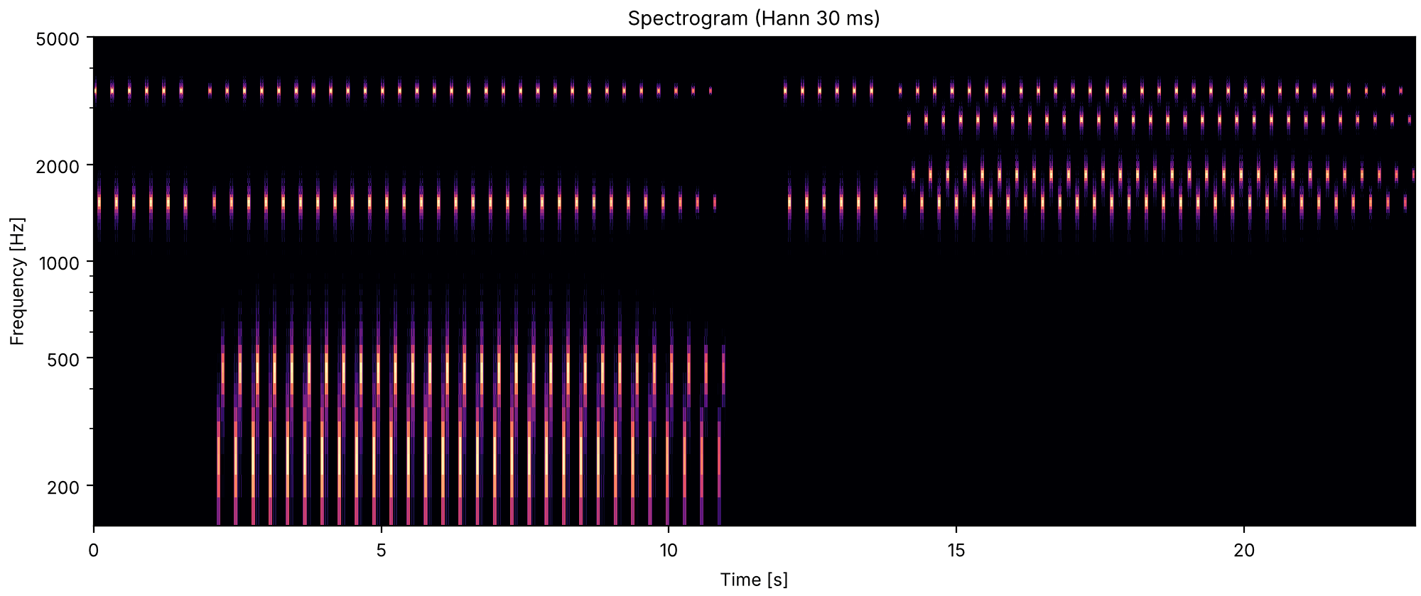
A and B, isolated or absorbed

Listen for the standard, A then B, inside the cycle: easy in the first cycle, hard in the second, where other tones near their pitches pull A and B away.

Bregman & Ahad, Demonstration 15, after Bregman (1978). A two-tone standard, A (3400 Hz) and B (1525 Hz) followed by two silences, then the four-tone cycle ABXY: 45 ms tones with 10 ms rises and decays and 30 ms silences, 300 ms a cycle, thirty cycles with a three-cycle fade-in and a ten-cycle fade-out. First X and Y low (246 and 455 Hz), then X near A and Y near B (2760 and 1860 Hz). The booklet reports the standard easy to hear in the first cycle, where A and B form a stream of their own, and hard in the second, where A goes with X and B with Y. How many cycles of the standard come first (six here) is ours.

sg12_a_and_b_isolated_or_absorbed.flac, 23.0 s, mono

Plots of the a and b, isolated or absorbed sound
Code
def cycle_of(freqs, n_cycles, start, fade=False):
    """`n_cycles` cycles of 45 ms tones 75 ms apart; with `fade`, a three-cycle fade-in and a
    ten-cycle fade-out."""
    gain = np.ones(n_cycles)
    if fade:
        gain = np.minimum(1, np.minimum((np.arange(n_cycles) + 1) / 3, (n_cycles - np.arange(n_cycles)) / 10))
    return [
        (start + 0.3 * c + 0.075 * k, so.Sound(gain[c] * tone(f, 0.045).data, FS))
        for c in range(n_cycles)
        for k, f in enumerate(freqs)
        if f
    ]


events = []
for start, (x, y) in ((0.0, (246, 455)), (12.0, (2760, 1860))):
    events += cycle_of((3400, 1525, None, None), 6, start)
    events += cycle_of((3400, 1525, x, y), 30, start + 2.0, fade=True)
sound = finish(place(events))
fig, playhead = show(sound, fmin=150, fmax=5000)

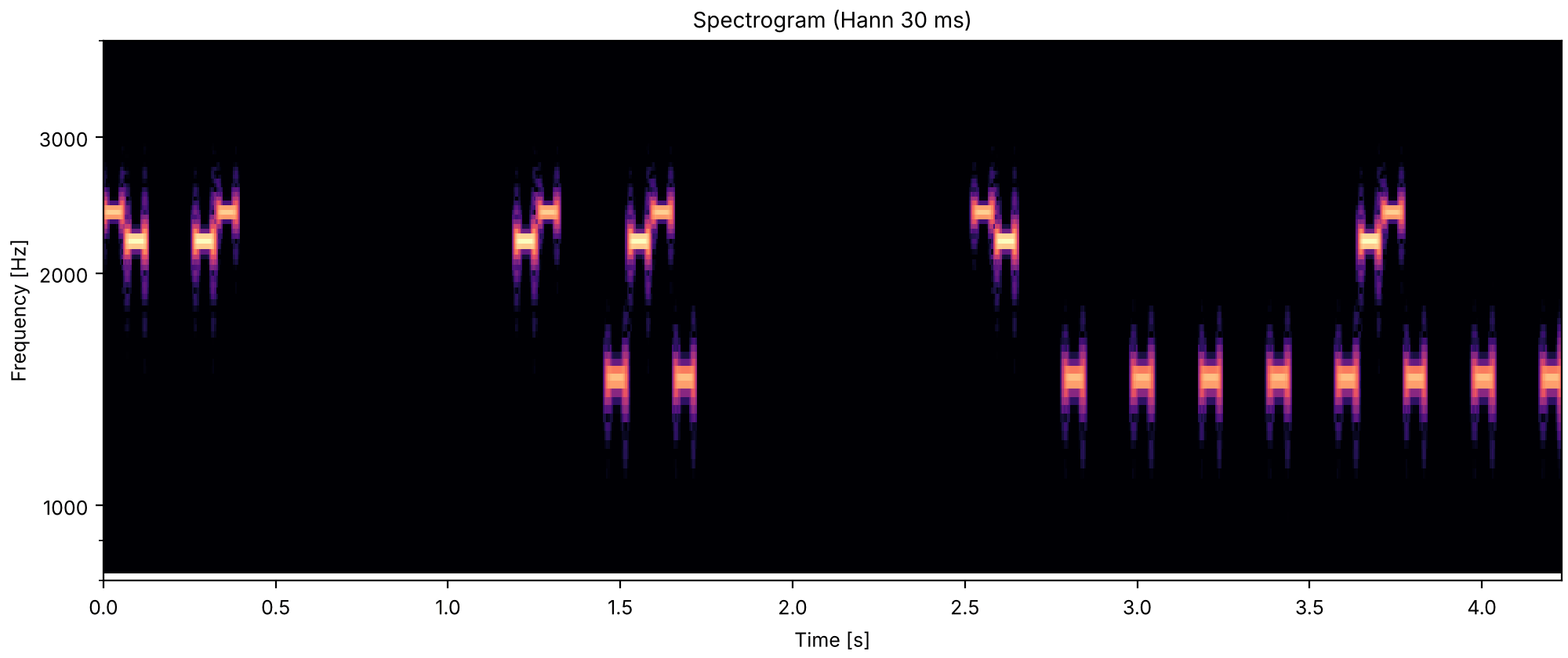
A two-tone order, hidden and freed

Listen for the order of the two high tones: clear alone, hard to hear between the lower X tones, and clear again when a run of captor tones pulls the X tones into a stream of their own.

Bregman & Ahad, Demonstration 16, after Bregman & Rudnicky (1975). Is A (2200 Hz) before B (2400 Hz), or after? Tones are 57 ms (7 ms rise, 5 ms decay) with 9 ms between them, and the 2400 and 1460 Hz tones are scaled by 0.5 and 0.4, as in the booklet. Three parts: the pair alone (BA then AB); a standard AB, then the pair between two 1460 Hz tones X (XABX), whose order the booklet reports is hard to hear; and a standard BA, then XABX inside a run of captor tones C at the same 1460 Hz and spacing, C--C--C--C--XABX--C--C, which the booklet reports frees A and B again. The silence between the parts (0.8 s) is ours.

sg13_a_two-tone_order_hidden_and_freed.flac, 4.2 s, mono

Plots of the a two-tone order, hidden and freed sound
Code
UNIT = 0.066
A = tone(2200, 0.057, 7e-3, 5e-3)
B = so.Sound(0.5 * tone(2400, 0.057, 7e-3, 5e-3).data, FS)
X = so.Sound(0.4 * tone(1460, 0.057, 7e-3, 5e-3).data, FS)
parts = ["BA  AB", "AB  XABX", "BA  C  C  C  C  XABX  C  C"]
events, t = [], 0.0
for part in parts:
    for symbol in part:
        if symbol != " ":
            events.append((t, {"A": A, "B": B, "X": X, "C": X}[symbol]))
        t += UNIT
    t += 0.8
sound = finish(place(events))
fig, playhead = show(sound, fmin=800, fmax=4000)

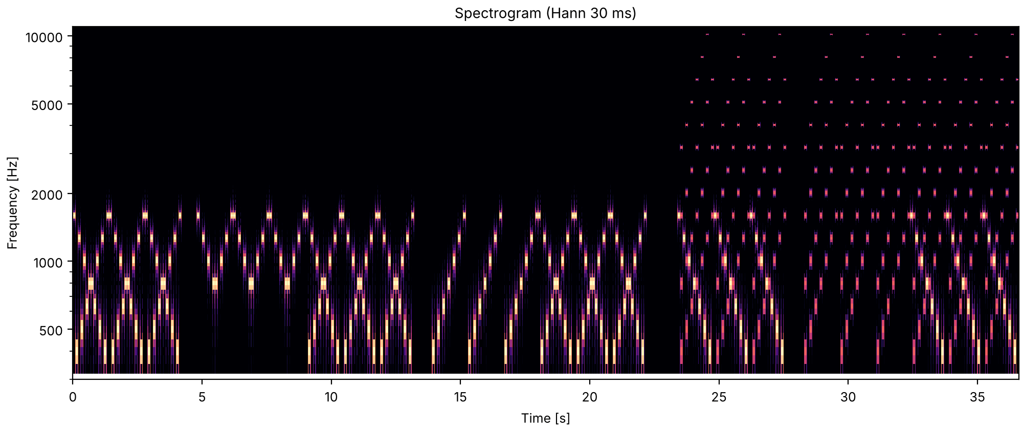
An X that bounces, and one that crosses

Listen for the path you follow through the X. With pure tones it tends to fall and then bounce back up, or rise and bounce down, rather than cross; once the rising tones are richer in timbre, the crossing line is easy to follow.

Bregman & Ahad, Demonstration 17, after Tougas & Bregman (1985). A rising sequence from 400 to 1600 Hz in seven equal log steps interleaved with the falling one, 100 ms tones with 10 ms rises and decays and no silences: an X. The booklet reports that listeners follow a path that bounces off the crossing (down then up, or up then down) rather than one that crosses, until the rising tones get a richer timbre (harmonics 1, 2, 4 and 8, each 20 dB below the pure tone). The disc then tests four standards against the X, before and after the change of timbre; this reproduction keeps two, the upper V (the falling tones above the crossing, then the rising ones) and the whole rising line, each as three cycles of standard then three of X, and after the change of timbre only the rising line. At this page's sample rate the eighth harmonic of the two highest rising tones does not fit and is left out.

sg14_an_x_that_bounces_and_one_that_crosses.flac, 36.6 s, mono

Plots of the an x that bounces, and one that crosses sound
Code
rising = 400 * 4 ** (np.arange(7) / 6)
falling = rising[::-1]


def pure(f):
    return tone(f, 0.1)


def rich(f):
    """Harmonics 1, 2, 4 and 8, each 20 dB below the pure tone; those above 11 kHz, which this
    sample rate cannot hold, are left out."""
    return so.Sound(sum(0.1 * tone(n * f, 0.1).data for n in (1, 2, 4, 8) if n * f < FS / 2), FS)


def x_pattern(rising_tone, keep, n_cycles, start):
    """`n_cycles` of the X, falling and rising tones in alternation, keeping those `keep` allows."""
    events = []
    for c in range(n_cycles):
        for k in range(7):
            for j, (f, make) in enumerate(((falling[k], pure), (rising[k], rising_tone))):
                if keep(f, j):
                    events.append((start + 1.4 * c + 0.2 * k + 0.1 * j, make(f)))
    return events


standards = {"upper V": lambda f, j: f >= 800, "rising line": lambda f, j: j == 1}
events, t = [], 0.0
for rising_tone, tests in ((pure, standards.values()), (rich, [standards["rising line"]])):
    events += x_pattern(rising_tone, lambda f, j: True, 3, t)
    t += 4.2 + 0.6
    for keep in tests:
        events += x_pattern(rising_tone, keep, 3, t) + x_pattern(rising_tone, lambda f, j: True, 3, t + 4.2)
        t += 8.4 + 0.6
    t += 0.6
sound = finish(place(events))
fig, playhead = show(sound, fmin=300, fmax=11000)

Interlocking parts

On the disc, Demonstrations 7 to 9 and 41 use a recording of East African xylophone (amadinda) music from Buganda, provided by Ulrich Wegner: two players each play an evenly spaced cycle of notes, interleaved, so that the listener hears high and low streams with rhythms that neither player plays. The recording is not ours to use, and neither is the piece's notation, so this section is a stand-in: two cycles of twelve notes drawn at random (seed 7) from a five-step scale of equal steps (240 cents) over two octaves from 220 Hz, played by a synthetic struck tone, 4.2 tones a second for each part as in the booklet. The struck tone is a fundamental with partials at 2.76 and 5.40 times it, the first modes of a free bar, decaying with a half-life of 25 ms, inside the booklet's 15 to 30 ms. It is not an amadinda, and the cycles are not the piece.

Two interleaved parts

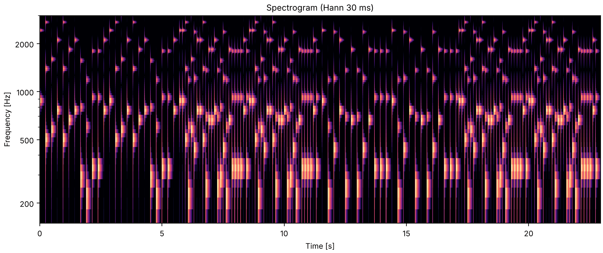
Listen for each part alone as an even beat with a simple tune; together, neither tune can be heard, and new rhythms appear.

After Bregman & Ahad, Demonstration 7. The first part alone, the second joining it, the second alone, both again, two cycles each. The booklet reports that when the parts play together, neither player's melody and even rhythm can be heard.

sg15_two_interleaved_parts.flac, 22.9 s, mono

Plots of the two interleaved parts sound
Code
SCALE = 220 * 2 ** (np.arange(11) * 240 / 1200)
rng = np.random.default_rng(7)
parts = [rng.integers(0, 11, 12), rng.integers(0, 11, 12)]
PERIOD = 1 / 4.2


def struck(freq, partials=(1, 2.76, 5.40), amps=(1, 0.3, 0.15), half_life=0.025):
    t = np.arange(round(0.2 * FS)) / FS
    env = np.minimum(1, t / 2e-3) * 0.5 ** (t / half_life)
    waves = sum(a * np.sin(2 * np.pi * p * freq * t) for p, a in zip(partials, amps, strict=True))
    return so.Sound(env * waves, FS)


def interlocking(plan, timbres=(struck, struck), octave=(0, 0), start=0.0, n_cycles=2):
    """`plan` lists which parts play in each block of `n_cycles` cycles."""
    events, t = [], start
    for playing in plan:
        for c in range(n_cycles):
            for k in range(12):
                for p in playing:
                    onset = t + (12 * c + k) * PERIOD + p * PERIOD / 2
                    events.append((onset, timbres[p](SCALE[parts[p][k]] * 2 ** octave[p])))
        t += 12 * n_cycles * PERIOD
    return events, t


events, _ = interlocking([(0,), (0, 1), (1,), (0, 1)])
sound = finish(place(events))
fig, playhead = show(sound, fmin=150, fmax=3000)

The second part an octave up

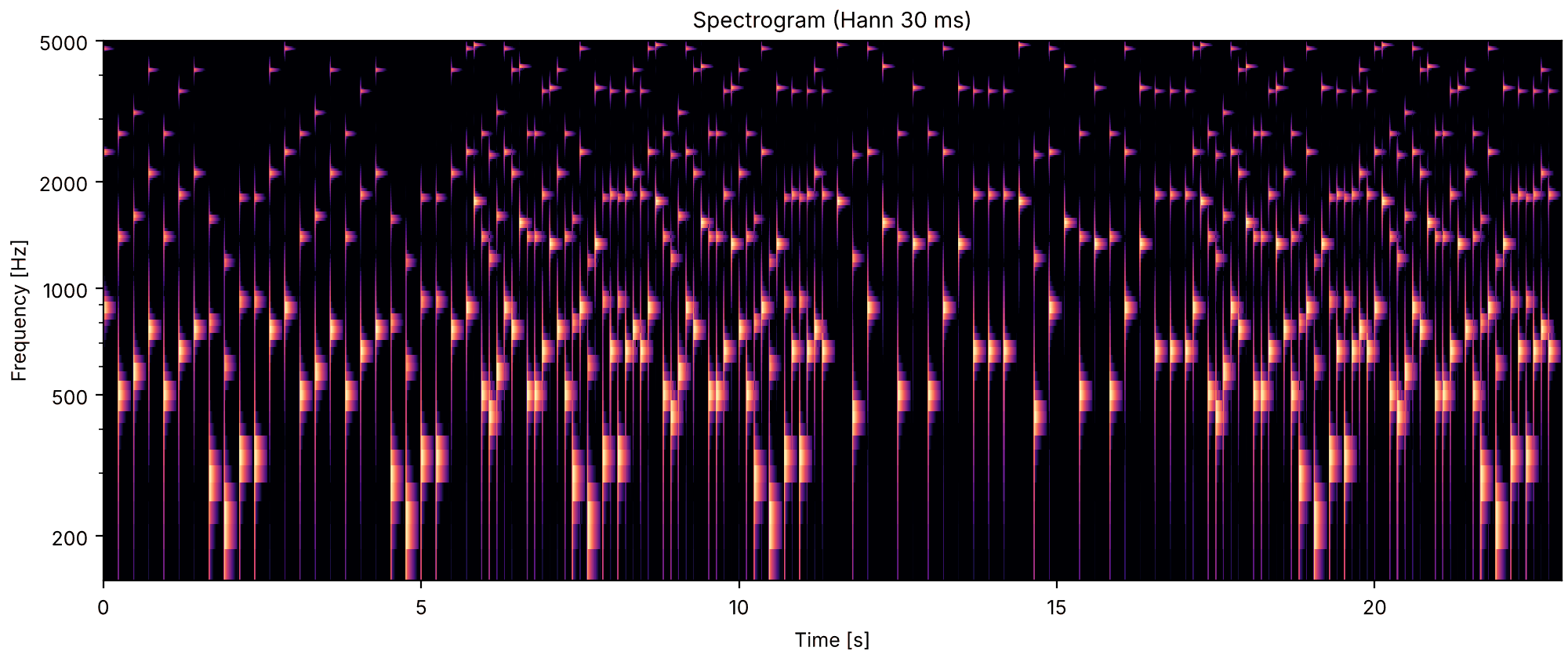
Listen for each part's own tune and even rhythm staying audible when they play together, now that the second part is an octave up.

After Bregman & Ahad, Demonstration 8. The same, with the second part an octave higher. The booklet reports that each player's part now stays audible with its own even rhythm when they play together.

sg16_the_second_part_an_octave_up.flac, 22.9 s, mono

Plots of the the second part an octave up sound
Code
events, _ = interlocking([(0,), (0, 1), (1,), (0, 1)], octave=(0, 1))
sound = finish(place(events))
fig, playhead = show(sound, fmin=150, fmax=5000)

The two parts in two timbres

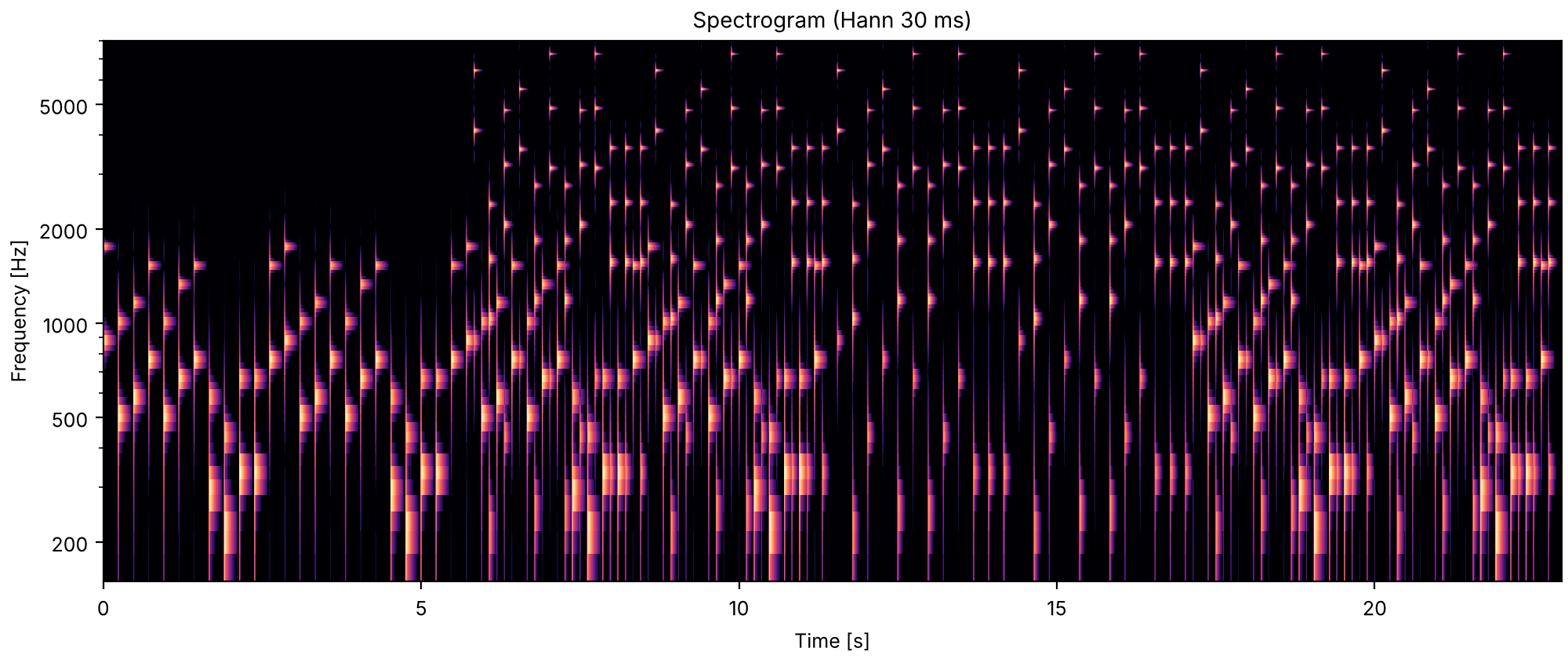
Listen for the two parts, in the same range again, separating by their timbres.

After Bregman & Ahad, Demonstration 9. The parts in the same range again, the first muffled (fundamental and second harmonic, as the booklet describes it) and the second brittle (strong high inharmonic partials and a weak fundamental). The booklet reports that the two parts split by timbre. The partials of both timbres are ours.

sg17_the_two_parts_in_two_timbres.flac, 22.9 s, mono

Plots of the the two parts in two timbres sound
Code
def muffled(f):
    return struck(f, partials=(1, 2), amps=(1, 0.5))


def brittle(f):
    return struck(f, partials=(1, 4.7, 7.3, 10.9), amps=(0.3, 1, 0.8, 0.6), half_life=0.015)


events, _ = interlocking([(0,), (0, 1), (1,), (0, 1)], timbres=(muffled, brittle))
sound = finish(place(events))
fig, playhead = show(sound, fmin=150, fmax=8000)

Place

Sounds from different sides split into streams, as sounds of different pitch do.

Noise bursts that move apart 🎧

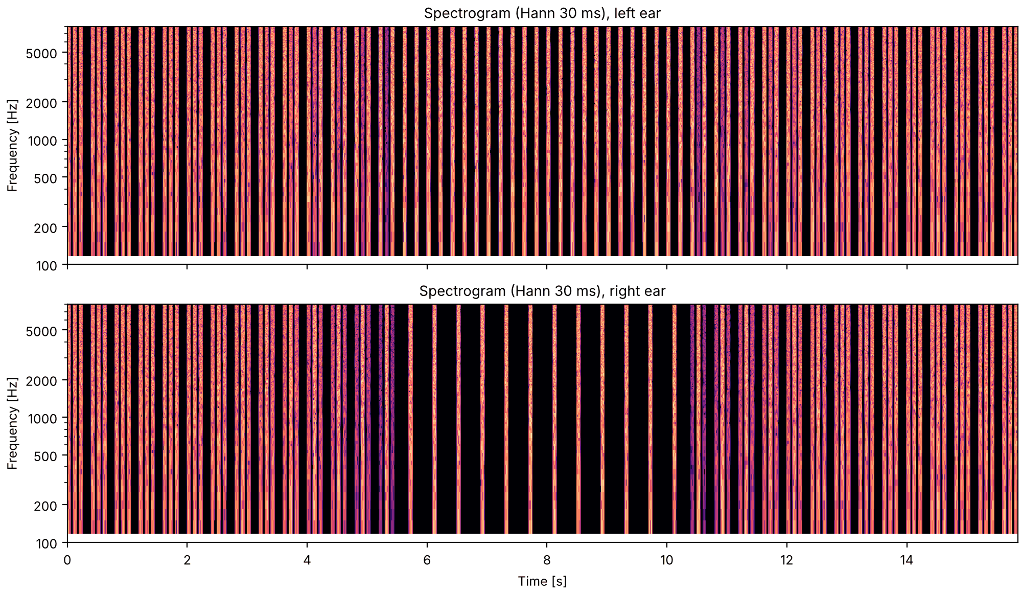
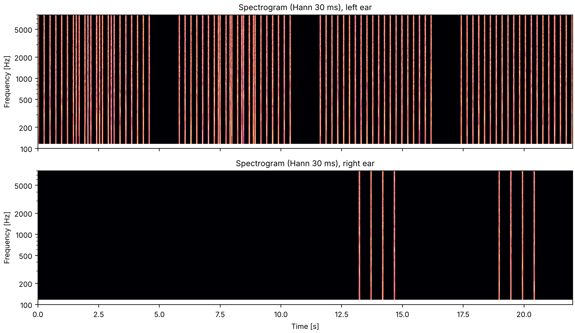
Listen for the gallop splitting into a fast beat on the left and a slow one on the right as the bursts move apart, and coming back when they return to the center.

Bregman & Ahad, Demonstration 38. Bursts of white noise in an ABA- gallop, 50 ms each with 1 ms onsets and offsets and 50 ms silences, so that A repeats every 200 ms and B every 400 ms. All start in the center (both ears equally); then A moves gradually into the left ear only and B into the right only, and back. The booklet reports that the gallop splits into a fast stream on the left and a slow one on the right, and returns when the bursts come back to the center. The booklet moves the bursts by level alone; how fast they move (over ten triplets, holding for ten) and the constant-power pan are ours, and the sequence plays once instead of twice.

sg18_noise_bursts_that_move_apart.flac, 15.9 s, stereo

Plots of the noise bursts that move apart sound
Code
rng = np.random.default_rng(38)
pan = np.concatenate([np.zeros(5), np.linspace(0, 1, 10), np.ones(10), np.linspace(1, 0, 10), np.zeros(5)])
events = []
for k, p in enumerate(pan):
    for j, side in enumerate((-1, 1, -1)):
        burst = so.gaussian_noise(0.05, FS, rng=rng).ramp(1e-3, shape="linear").data[:, 0]
        angle = np.pi / 4 * (1 + side * p)
        pair = np.column_stack([np.cos(angle) * burst, np.sin(angle) * burst])
        events.append((0.4 * k + 0.1 * j, so.Sound(pair, FS)))
sound = finish(place(events))
fig, playhead = show(sound, fmin=100, fmax=8000)

A middle burst on time or late 🎧

Listen for whether the middle burst is late: easy to hear with everything in one ear, harder with B in the other ear.

Bregman & Ahad, Demonstration 39. 40 ms bursts of white noise, A then B then A, with 200 ms from the end of one A to the start of the next; B either sits in the middle (80 ms of silence on each side) or is late (130 ms before it, 30 after). Each gallop is framed by A bursts alone. First everything in the left ear, B in the middle and then late; then A in the left ear and B in the right, B late and then in the middle (the order the booklet's answer gives). The booklet reports the late B harder to notice when it comes from the other side. The number of bursts (six A alone before and after, eight triplets) is ours.

sg19_a_middle_burst_on_time_or_late.flac, 22.0 s, stereo

Plots of the a middle burst on time or late sound
Code
rng = np.random.default_rng(39)


def burst(ear):
    data = so.gaussian_noise(0.04, FS, rng=rng).ramp(1e-3, shape="linear").data[:, 0]
    return so.Sound(np.column_stack([data * (ear == "left"), data * (ear == "right")]), FS)


events, t = [], 0.0
for b_ear, delays in (("left", (0.08, 0.13)), ("right", (0.13, 0.08))):
    for delay in delays:
        for k in range(6 + 8 + 6):
            events.append((t, burst("left")))
            if 6 <= k < 14 and (k - 6) % 2 == 0:
                events.append((t + 0.04 + delay, burst(b_ear)))
            t += 0.24
        t += 1.0
sound = finish(place(events))
fig, playhead = show(sound, fmin=100, fmax=8000)

The two parts moving apart 🎧

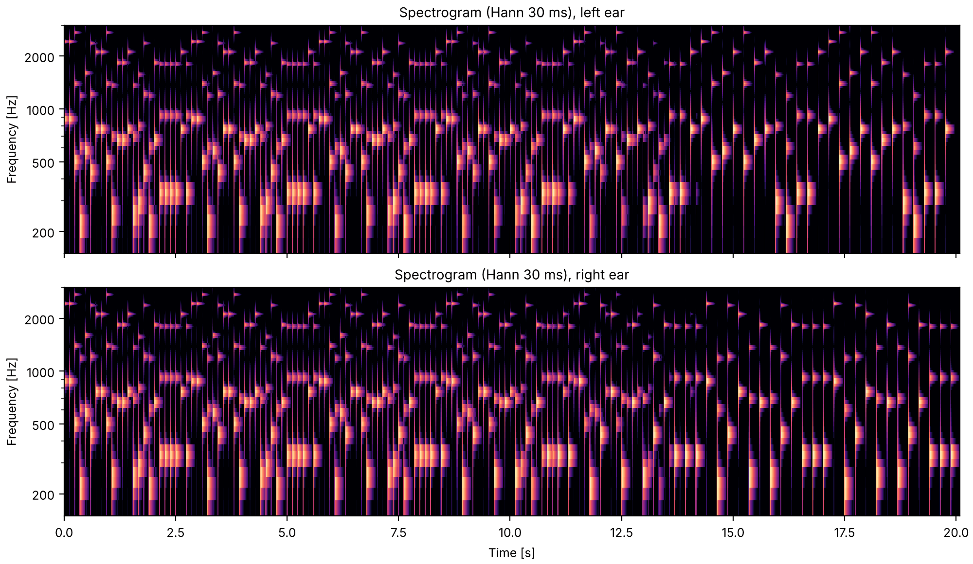
Listen for the two parts, once in opposite ears, each heard with its own even rhythm.

After Bregman & Ahad, Demonstration 41. The interleaved parts of the stand-in above, first sent equally to both ears for two cycles, then moving apart over three, the first part to the left and the second to the right, and apart for two more. The booklet reports that the parts, once apart, are heard each with its own even rhythm.

sg20_the_two_parts_moving_apart.flac, 20.1 s, stereo

Plots of the the two parts moving apart sound
Code
events, end = interlocking([(0, 1)], n_cycles=7)
stereo = []
for onset, snd in events:
    first_part = round(onset / (PERIOD / 2)) % 2 == 0
    p = np.clip((onset - 2 * 12 * PERIOD) / (3 * 12 * PERIOD), 0, 1)
    angle = np.pi / 4 * (1 + (-1 if first_part else 1) * p)
    pair = np.column_stack([np.cos(angle) * snd.data[:, 0], np.sin(angle) * snd.data[:, 0]])
    stereo.append((onset, so.Sound(pair, FS)))
sound = finish(place(stereo))
fig, playhead = show(sound, fmin=150, fmax=3000)

References

  • Bregman & Ahad (1996). Demonstrations of Auditory Scene Analysis: The Perceptual Organization of Sound (compact disc and booklet). Auditory Perception Laboratory, McGill University; MIT Press. Recordings and booklet.
  • Houtsma, Rossing & Wagenaars (1987). Auditory Demonstrations (compact disc and booklet). Institute for Perception Research (IPO), Eindhoven, and the Acoustical Society of America. Booklet.
  • Bregman (1978). Auditory streaming: competition among alternative organizations. Perception & Psychophysics 23, 391–398. doi:10.3758/BF03204141.
  • Bregman (1990). Auditory Scene Analysis: The Perceptual Organization of Sound. MIT Press. doi:10.7551/mitpress/1486.001.0001.
  • Bregman & Campbell (1971). Primary auditory stream segregation and perception of order in rapid sequences of tones. J. Exp. Psychol. 89(2), 244–249. doi:10.1037/h0031163.
  • Bregman & Dannenbring (1973). The effect of continuity on auditory stream segregation. Perception & Psychophysics 13, 308–312. doi:10.3758/BF03214144.
  • Bregman & Rudnicky (1975). Auditory segregation: stream or streams? J. Exp. Psychol.: Human Perception and Performance 1(3), 263–267. doi:10.1037/0096-1523.1.3.263.
  • Dannenbring & Bregman (1976). Stream segregation and the illusion of overlap. J. Exp. Psychol.: Human Perception and Performance 2(4), 544–555. doi:10.1037/0096-1523.2.4.544.
  • Dowling (1973). The perception of interleaved melodies. Cognitive Psychology 5(3), 322–337. doi:10.1016/0010-0285(73)90040-6.
  • Peterson & Barney (1952). Control methods used in a study of the vowels. J. Acoust. Soc. Am. 24(2), 175–184.
  • Tougas & Bregman (1985). Crossing of auditory streams. J. Exp. Psychol.: Human Perception and Performance 11(6), 788–798. doi:10.1037/0096-1523.11.6.788.
  • van Noorden (1975). Temporal Coherence in the Perception of Tone Sequences. Doctoral thesis, Eindhoven University of Technology. TU/e.

The original papers were checked for their titles and publication details; the stimulus parameters on this page come from Bregman & Ahad's and Houtsma et al.'s booklets, not from the papers.