Continuity and capture: reproducing Bregman & Ahad

Every sound on this page is sonore's reproduction of a published demonstration. All but one are from Albert Bregman and Pierre Ahad's Demonstrations of Auditory Scene Analysis (1996), the compact disc that accompanies Bregman's book Auditory Scene Analysis (1990); one, the pulsation threshold, is from the Acoustical Society of America's Auditory Demonstrations (Houtsma, Rossing & Wagenaars, 1987). The demonstrations, their design and what they show are their authors' work. Bregman's laboratory publishes the original recordings and booklet (McGill), and they are the ones to listen to.

What they show. When a sound suddenly gets louder or richer, hearing tends to take the change as the old sound carrying on with a new sound added on top. Bregman calls this the old-plus-new heuristic. It has three consequences that the examples below make audible. A tone heard just before a mixture can capture its match out of the mixture, so the mixture loses that part. A soft sound cut off by a louder sound that could have hidden it is heard continuing behind the loud one. And what is left of the mixture once the old sound is taken out, the residual, is heard as a new sound of its own. Streams is about sounds grouped one after another and Fusion about sounds grouped at the same time; this page is about the two kinds of grouping competing. Each example opens with what to listen for, taken from what the booklet reports listeners hear.

This page is a test of sonore: can its generators rebuild each stimulus from the description in the booklet? Each example names the demonstration it reproduces, rebuilds it from the booklet's frequencies, levels and timing, and says where it departs from them: where the booklet leaves a value open, where a recording is replaced by a stand-in, or where a long track is shortened. What listeners hear is reported as the booklet reports it; this page has not tested any of it.

  • Capturing a tone out of a mixture: a tone pulled out of a two-tone chord by the tones before it (Bregman & Ahad, Demonstrations 25 to 27).
  • Continuing through noise: tones, glides and speech heard carrying on behind loud noise (Demonstrations 28 to 32; Houtsma et al., Demonstration 11).
  • What is left over: the residual heard as a sound of its own (Demonstrations 33 to 35).
  • Glides and a vowel: capturing a glide out of a mixture of glides, and changing a vowel by capturing one of its harmonics (Demonstrations 36 and 37).
Setup, the same on every page
import os
import urllib.request

import matplotlib.pyplot as plt
import numpy as np

import sonore as so

plt.rcParams.update({"font.size": 9, "axes.titlesize": 10, "figure.dpi": 100})


def fetch(path):
    """A file from the sonore repository, by its path there: the local copy when this runs from
    the repository root, otherwise downloaded from GitHub to the same relative path."""
    if not os.path.exists(path):
        os.makedirs(os.path.dirname(path) or ".", exist_ok=True)
        urllib.request.urlretrieve("https://raw.githubusercontent.com/choyun1/sonore/main/" + path, path)
    return path


def finish(snd):
    """How every sound in the gallery is played: 5 ms ramps, RMS 0.1, peak at most 0.95."""
    snd = snd.ramp(5e-3).normalize(rms=0.1)
    return snd.normalize(peak=0.95) if snd.peak > 0.95 else snd

Press play and a line follows the sound across every time axis in its plots. Click any time axis to play from that point. Start with your volume low.

To run this page yourself, open it as a notebook in Colab or download it. It is the same code, and it fetches the recordings it needs from the sonore repository.

Code the examples share

The tones are placed at their onset times, as on the Streams page; tones and noises that switch on and off over a longer sound are multiplied by on, a level that is 1 inside given stretches of time and 0 outside them. Like every sonore generator, so.pure_tone, so.harmonic_complex and so.gaussian_noise scale the sound they make to RMS 1, so each pure tone and each glide here has RMS 1 and the booklets' level relations are set by scaling from there. finish keeps those relations, scaling only the whole sound. The sample rate is 22.05 kHz, except for the speech, which keeps its recording's 16 kHz.

Code
FS = 22050


def envelope(n, rise, decay):
    """Linear rise and decay ramps, in seconds, over `n` samples."""
    i = np.arange(n)
    return np.clip(np.minimum(i / (rise * FS), (n - 1 - i) / (decay * FS)), 0, 1)


def tone(freq, dur, rise=10e-3, decay=10e-3):
    """A sine tone at RMS 1 (before its ramps), `dur` seconds long including linear ramps."""
    snd = so.pure_tone(dur, FS, freq, phase=-np.pi / 2)
    return so.Sound(envelope(snd.n_samples, rise, decay) * snd.data[:, 0], FS)


def place(events, dur=None):
    """Sounds added at their onset times: `events` is a list of (onset in seconds, Sound)."""
    end = max(onset + snd.duration for onset, snd in events)
    out = np.zeros((round((dur or end) * FS) + 1, 1))
    for onset, snd in events:
        i = round(onset * FS)
        out[i : i + snd.n_samples] += snd.data[: len(out) - i]
    return so.Sound(out, FS)


def on(t, starts, length, ramp=5e-3):
    """1 for `length` seconds from each of `starts` and 0 elsewhere, changing along straight ramps
    `ramp` seconds long centered on each edge (abruptly if `ramp` is 0). One minus it is 1 exactly
    where it is not, so a sound gated by `on` and another by `1 - on` cross-fade."""
    level = np.zeros_like(t)
    for start in starts:
        if ramp:
            level += np.clip(np.minimum(t - start, start + length - t) / ramp + 0.5, 0, 1)
        else:
            level += (t >= start) & (t < start + length)
    return level


def glide(f_start, dur, octaves_per_second, ramp=10e-3):
    """A pure glide at RMS 1 (before its ramps), straight on a log-frequency axis, from `f_start`
    for `dur` seconds, with linear ramps."""
    times = np.linspace(0, dur, 101)
    contour = (times, f_start * 2 ** (octaves_per_second * times))
    snd = so.harmonic_complex(dur, FS, contour, harmonics=[1], ramp=0)
    return so.Sound(envelope(snd.n_samples, ramp, ramp) * snd.data[:, 0], FS)


def show(snd, fmin=100, fmax=5000, title="Spectrogram (Hann 30 ms)", log=True):
    """A spectrogram, on a log frequency axis unless `log` is False. Returns the figure and the
    panels the playhead follows."""
    fig, ax = plt.subplots(figsize=(10, 3.2), layout="constrained")
    stft = so.STFT(snd, win_dur=30e-3, hop_dur=5e-3)
    keep = (stft.f >= fmin) & (stft.f <= fmax)
    top = stft.db[:, keep].max()
    ax.pcolormesh(stft.t, stft.f[keep], stft.db[0][keep], vmin=top - 60, vmax=top, cmap="magma")
    if log:
        so.plotting.log_frequency_axis(ax)
    ax.set(ylim=(fmin, fmax), ylabel="Frequency [Hz]", title=title)
    ax.set(xlabel="Time [s]", xlim=(0, snd.duration))
    return fig, [ax]

Capturing a tone out of a mixture

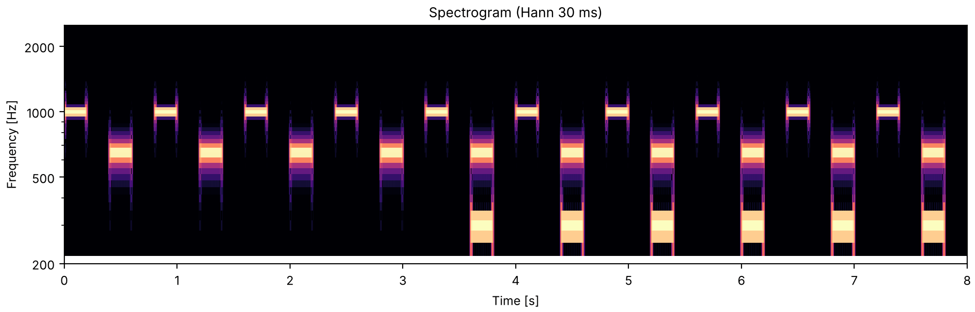
Two tones that start and stop together tend to fuse into one sound. A tone heard just before them, close in frequency to one of the two, can pull that one away into a stream of its own. Which grouping wins depends on how strong each pull is.

A far above the chord

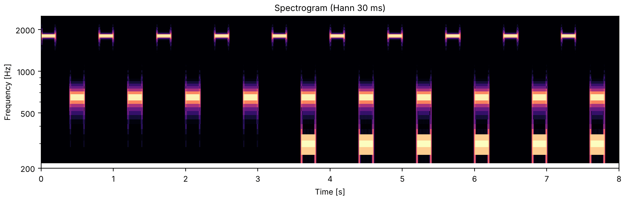
Listen for the high tone A and the upper tone B of the chord: can you keep hearing the alternating A B A B of the opening (the standard) once the low tone C joins B? Here A is at 1800 Hz, far above B, and the booklet expects B to fuse with C into one richer tone that alternates with a pure A. The next two sounds bring A closer to B.

Bregman & Ahad, Demonstration 25, a pattern discussed in Bregman (1990). Pure tones of equal amplitude: B at 650 Hz and C at 300 Hz always, and A at 1800, 1200 or 650 Hz in the three examples. Tones and the silences between them are 200 ms long, the tones with 10 ms rise and decay, so the cycle is A, silence, B and C together, silence. Four cycles of the standard (A and B alone) come first, as in the booklet, then six of the full pattern, where the booklet plays twelve. The booklet reports that the closer A is to B, the more easily B is heard going with A rather than with C.

cc1_a_far_above_the_chord.flac, 8.0 s, mono
Plots of the a far above the chord sound
Code
CYCLE = 0.8


def capture(a, b=650, c=300, c_delay=0.0, n_standard=4, n_full=6):
    """The A, B-and-C cycle after its A-B standard; C starts and stops `c_delay` seconds after B."""
    events = []
    for k in range(n_standard + n_full):
        start = CYCLE * k
        events += [(start, tone(a, 0.2)), (start + 0.4, tone(b, 0.2))]
        if k >= n_standard:
            events.append((start + 0.4 + c_delay, tone(c, 0.2)))
    return place(events, dur=CYCLE * (n_standard + n_full))


sound = finish(capture(1800))
fig, playhead = show(sound, fmin=200, fmax=2500)
A nearer the chord

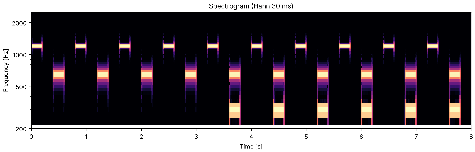
Listen for the same question with A at 1200 Hz, nearer to B.

Bregman & Ahad, Demonstration 25, its second example, built as the first.

cc1b_a_nearer_the_chord.flac, 8.0 s, mono

Plots of the a nearer the chord sound
Code
sound = finish(capture(1200))
fig, playhead = show(sound, fmin=200, fmax=2500)
A the same as B

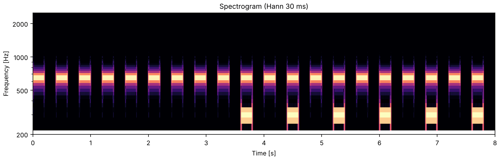
Listen for the same question with A at 650 Hz, the same as B: the standard is one repeated tone, and the booklet reports that B goes with A into a stream of identical pure tones, leaving C on its own as a low tone.

Bregman & Ahad, Demonstration 25, its third example, built as the first.

cc1c_a_the_same_as_b.flac, 8.0 s, mono

Plots of the a the same as b sound
Code
sound = finish(capture(650))
fig, playhead = show(sound, fmin=200, fmax=2500)
B and C together

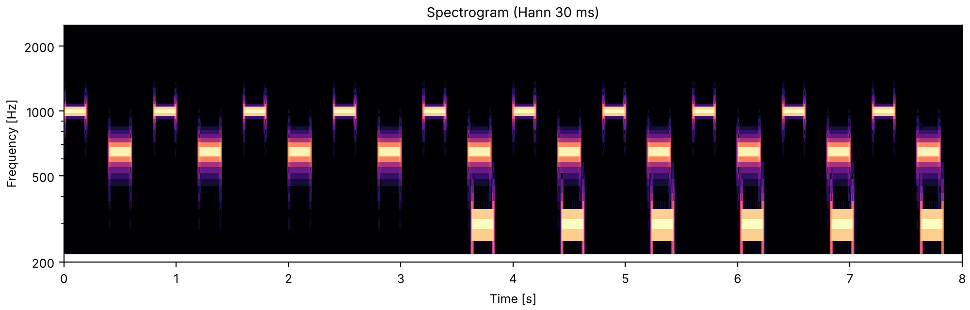
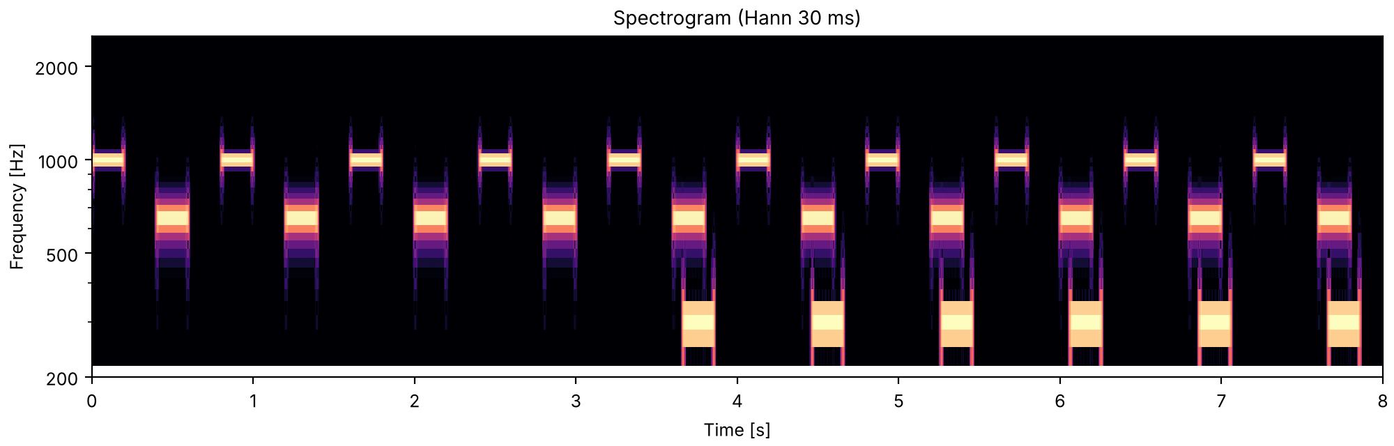
Listen for how easily you can keep hearing the standard's A B A B once C joins. Here B and C start and stop together. In the next two sounds C starts and stops later than B, and the booklet reports that the later it comes, the less B fuses with it and the more easily B is heard with A.

Bregman & Ahad, Demonstration 26. As Demonstration 25 with A at 1000 Hz, B at 650 Hz and C at 300 Hz, so that A and B are 350 Hz apart, a distance the booklet chose to leave the two pulls balanced. Both the onset and the offset of C are delayed by 0, 30 or 60 ms relative to B in the three examples. Four cycles of the standard, then six of the full pattern (the booklet plays twelve), as on the previous example.

cc2_b_and_c_together.flac, 8.0 s, mono

Plots of the b and c together sound
Code
sound = finish(capture(1000))
fig, playhead = show(sound, fmin=200, fmax=2500)
C 30 ms after B

Listen for the same question with C starting and stopping 30 ms after B.

Bregman & Ahad, Demonstration 26, its second example.

cc2b_c_30_ms_after_b.flac, 8.0 s, mono

Plots of the c 30 ms after b sound
Code
sound = finish(capture(1000, c_delay=0.03))
fig, playhead = show(sound, fmin=200, fmax=2500)
C 60 ms after B

Listen for the same question with C starting and stopping 60 ms after B.

Bregman & Ahad, Demonstration 26, its third example.

cc2c_c_60_ms_after_b.flac, 8.0 s, mono

Plots of the c 60 ms after b sound
Code
sound = finish(capture(1000, c_delay=0.06))
fig, playhead = show(sound, fmin=200, fmax=2500)
A fourth tone that frees the chord

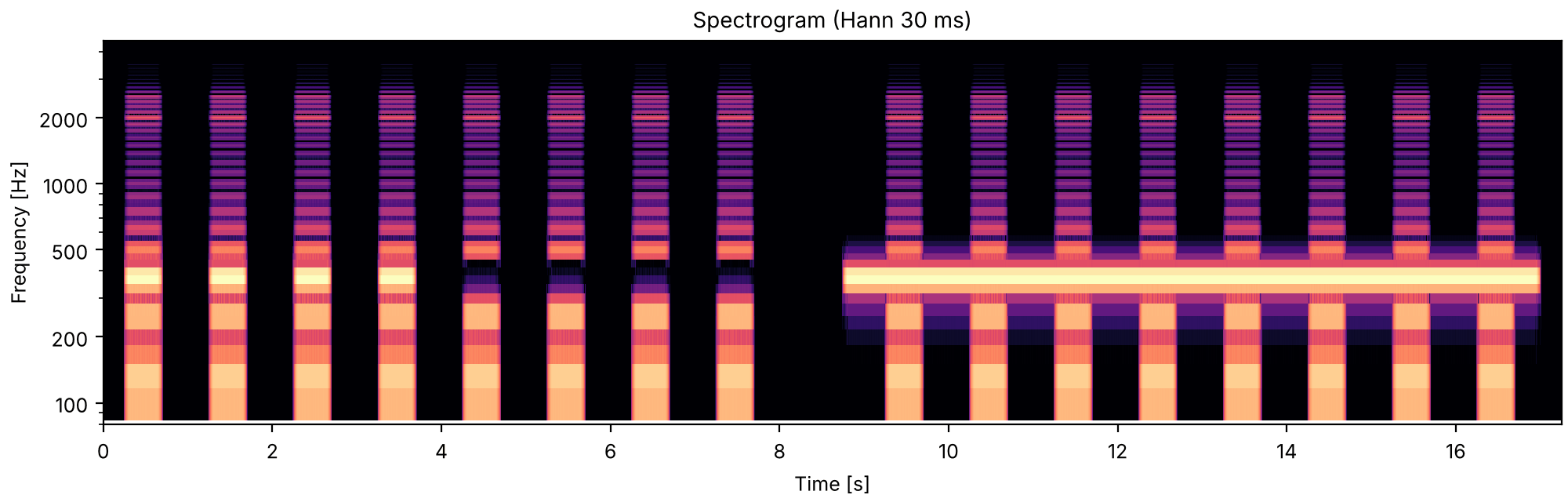
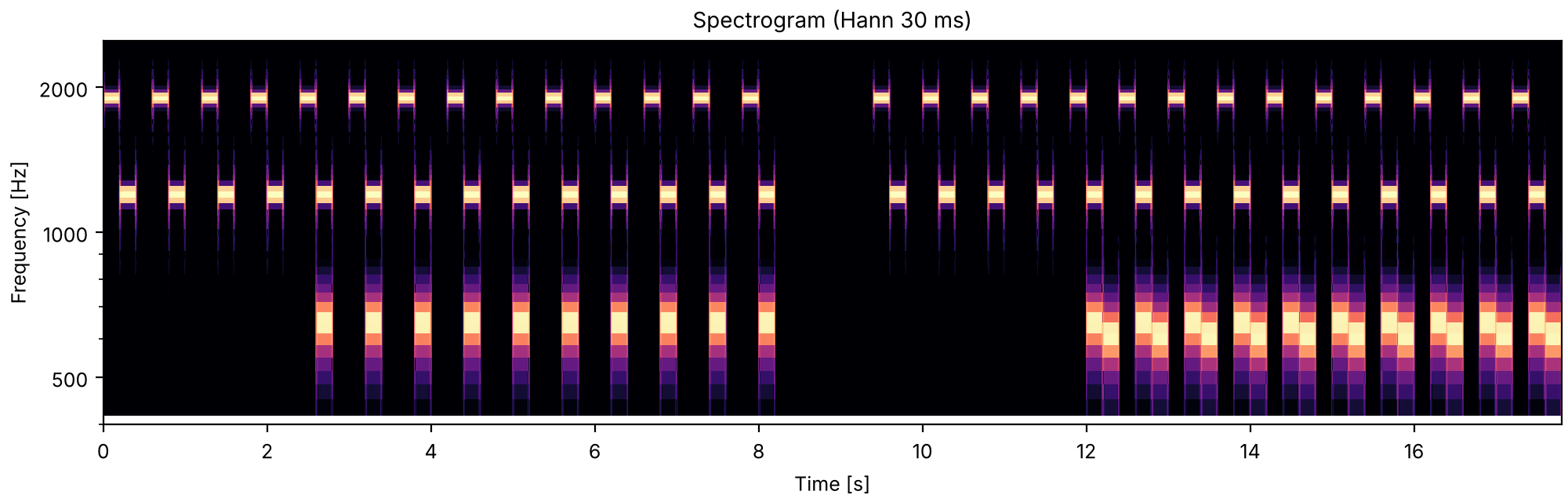
Listen for the standard, A B, inside each of the two patterns that follow it. In the first the chord is followed by a silence; in the second it is followed by a fourth tone D, just below C. The booklet reports that A and B are easier to hear together in the second pattern: D pulls C into a stream of its own, which loosens C's hold on B, so B is freer to go with A, although neither A nor B has changed.

Bregman & Ahad, Demonstration 27, after Bregman & Tougas (1989). Pure tones of equal amplitude, 200 ms long with 10 ms rise and decay: A 1900, B 1200, C 650 and D 613 Hz, with no silences between A, the chord of B and C, and D (or the silence in its place), all as in the booklet. Ours: the number of cycles (four of the standard, then ten of each pattern) and the 1 s pause between the two.

cc3_a_fourth_tone_that_frees_the_chord.flac, 17.8 s, mono

Plots of the a fourth tone that frees the chord sound
Code
def with_or_without_d(d, start):
    events = []
    for k in range(14):
        t = start + 0.6 * k
        events += [(t, tone(1900, 0.2)), (t + 0.2, tone(1200, 0.2))]
        if k >= 4:
            events.append((t + 0.2, tone(650, 0.2)))
            if d:
                events.append((t + 0.4, tone(613, 0.2)))
    return events


sound = finish(place(with_or_without_d(False, 0.0) + with_or_without_d(True, 9.4)))
fig, playhead = show(sound, fmin=400, fmax=2500)

Continuing through noise

A soft sound cut off by a burst of louder noise is heard carrying on behind the noise, as long as the noise could have hidden it. With a silence in the cut instead, the sound is heard stopping and starting.

A tone and a noise in its gap

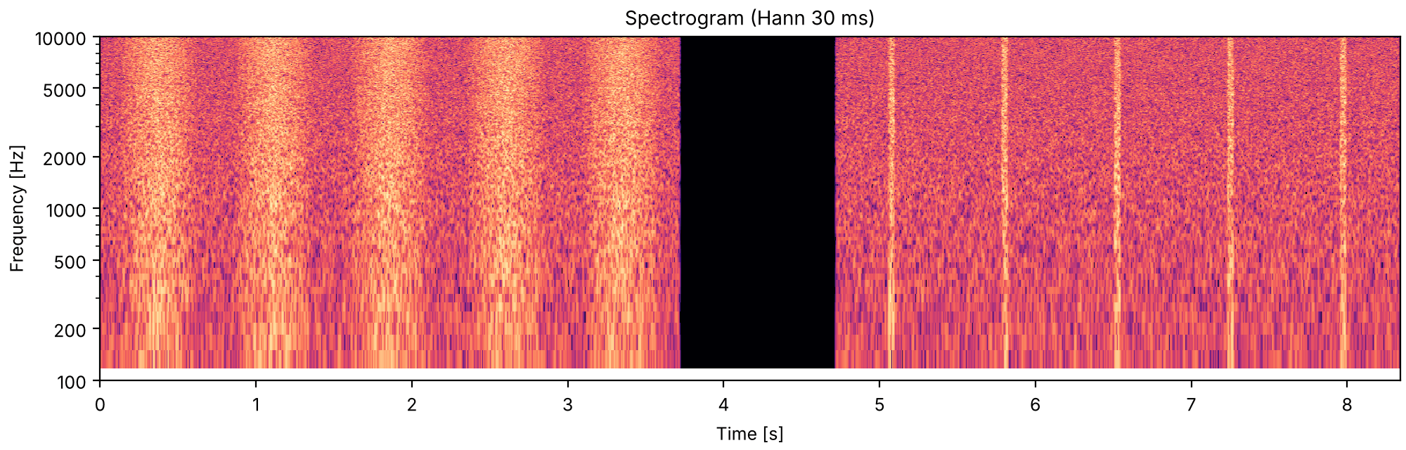
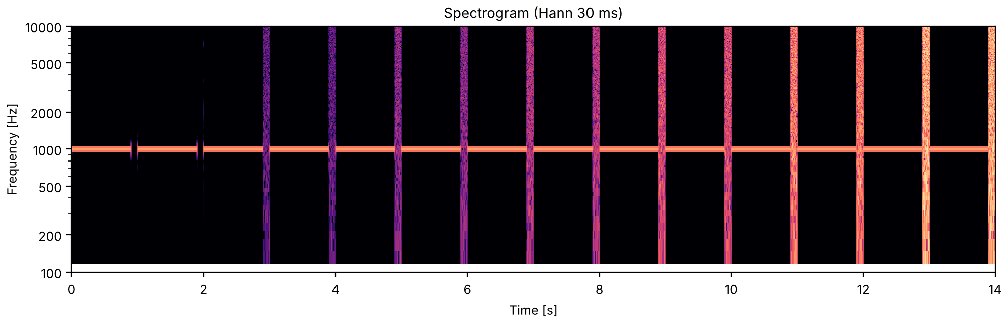
Listen for a steady tone that breaks off for a tenth of a second every second. The gap holds silence at first, then a burst of noise that gets louder in steps. The booklet reports that at the loudest step the tone seems to stay on behind the noise without a break, and invites you to judge whether it does at any of the earlier steps.

Bregman & Ahad, Demonstration 28, after Warren (1982). A 1000 Hz tone for 900 ms alternating with 100 ms of white noise, with the noise's amplitude stepping through 0, 0.025, 0.05, 0.1, 0.2, 0.5 and 1 of its final level. At the final level the booklet gives the noise's overall amplitude as about 20 times the tone's, which is the RMS ratio here. Ours: two cycles at each level (the booklet does not give the number) and cross-fades of 5 ms between tone and noise.

cc4_a_tone_and_a_noise_in_its_gap.flac, 14.0 s, mono

Plots of the a tone and a noise in its gap sound
Code
t = np.arange(round(14 * FS)) / FS
gaps = on(t, 0.9 + np.arange(14), 0.1)
steps = np.repeat([0, 0.025, 0.05, 0.1, 0.2, 0.5, 1], 2)
noise_level = 20 * steps[np.minimum(t.astype(int), 13)]
noise = so.gaussian_noise(14, FS, rng=np.random.default_rng(28)).data[: len(t), 0]
tone_1000 = so.pure_tone(14, FS, 1000).data[: len(t), 0]
sound = finish(so.Sound((1 - gaps) * tone_1000 + gaps * noise_level * noise, FS))
fig, playhead = show(sound, fmin=100, fmax=10000)

A tone stepping down between noise bursts

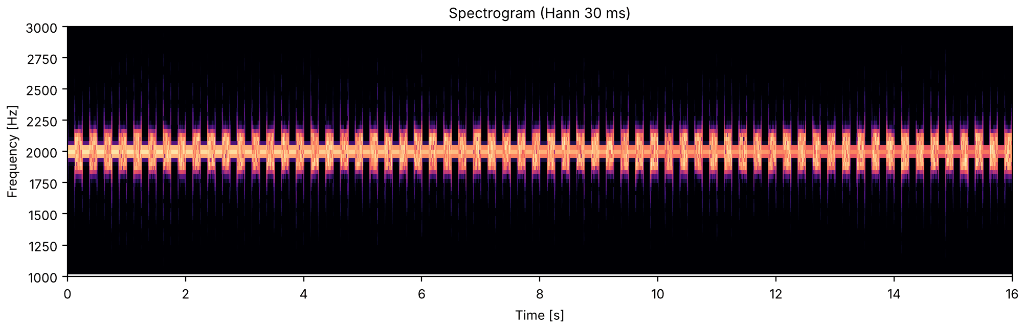
Listen for a tone that alternates with a narrow band of noise around its own frequency, and softens one step every four tones. At first the tone is heard pulsing on and off; the booklet reports that below some level, the pulsation threshold, it seems to sound on continuously through the noise.

Houtsma, Rossing & Wagenaars, Demonstration 11, after Houtgast (1972). A 2000 Hz tone for 125 ms alternating with 125 ms of noise from 1875 to 2125 Hz. The tone starts at the noise's level and drops 1 dB after every four tones, in 15 steps, while the noise stays the same, all as in the booklet. The cross-fades of 5 ms are ours; the booklet plays the series once and so does this reproduction.

cc5_a_tone_stepping_down_between_noise_bursts.flac, 16.0 s, mono

Plots of the a tone stepping down between noise bursts sound
Code
t = np.arange(round(16 * FS)) / FS
noise_slots = on(t, 0.125 + 0.25 * np.arange(64), 0.125)
tone_db = -np.floor(t / 1.0)  # four tones a second, 1 dB down after every four
band = so.gaussian_noise(16, FS, band=(1875, 2125), rng=np.random.default_rng(11)).data[: len(t), 0]
tone_2000 = so.pure_tone(16, FS, 2000).data[: len(t), 0]
sound = finish(so.Sound((1 - noise_slots) * 10 ** (tone_db / 20) * tone_2000 + noise_slots * band, FS))
fig, playhead = show(sound, fmin=1000, fmax=3000, log=False)

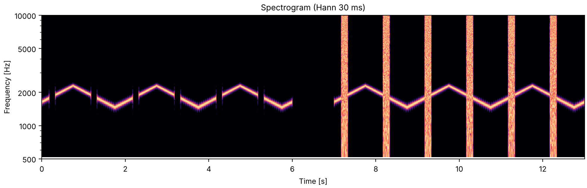
A glide cut in the middle of its rises and falls

Listen for a tone gliding up and down, with a short piece cut out of the middle of every rise and every fall. For the first three cycles the cuts are silent; then they hold loud noise, and the booklet reports the glide heard as complete, carrying on behind the noise.

Bregman & Ahad, Demonstration 29, after Dannenbring (1976). A pure tone gliding between 1464 and 2297 Hz, straight on a log-frequency axis, a full cycle up and down taking 2 s. The cuts are 0.15 s long; the noise is white with a peak amplitude 21 times the tone's, all as in the booklet. Ours: three cycles of each, and cross-fades of 5 ms.

cc6_a_glide_cut_in_the_middle_of_its_rises_and_falls.flac, 13.0 s, mono

Plots of the a glide cut in the middle of its rises and falls sound
Code
LOW, HIGH = 1464, 2297
t = np.arange(round(6 * FS)) / FS
times = np.linspace(0, 6, 6001)
triangle = 1 - np.abs((times + 0.25) % 2 - 1)  # 0 at the bottom, 1 at the top; starts on the way up
glide_tone = so.harmonic_complex(6, FS, (times, LOW * (HIGH / LOW) ** triangle), harmonics=[1], ramp=0)
glide_tone = glide_tone.data[: len(t), 0]
rng = np.random.default_rng(29)


def cut_glide(centers, width, noise):
    """The glide with `width`-second cuts around `centers`, filled with noise if `noise`."""
    cuts = on(t, np.asarray(centers) - width / 2, width)
    filler = 0
    if noise:
        burst = so.gaussian_noise(6, FS, rng=rng).data[: len(t), 0]
        peak = max(np.abs(burst[cuts > 0.5 * (cuts.max())]).max(), 1e-9)
        filler = 21 * np.sqrt(2) * burst / peak  # the tone's peak is sqrt(2)
    return so.Sound((1 - cuts) * glide_tone + cuts * filler, FS).ramp(10e-3)


def silent_then_noise(centers, width):
    return so.concat([cut_glide(centers, width, False), so.silence(1.0, FS), cut_glide(centers, width, True)])


mid_legs = 0.25 + np.arange(6)  # halfway up and halfway down, in this sound's time
sound = finish(silent_then_noise(mid_legs, 0.15))
fig, playhead = show(sound, fmin=500, fmax=10000)

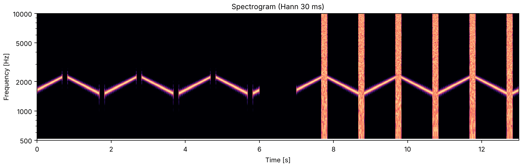
A glide cut where it turns

Listen for the same glide, now cut at its tops and bottoms, where it turns: silent cuts first, then noise. The booklet reports the glide heard turning behind the noise. It takes this as a sign that hearing does not simply copy what came before the noise but makes a guess about what went on during it.

Bregman & Ahad, Demonstration 29, its second part, built as the first.

cc6b_a_glide_cut_where_it_turns.flac, 13.0 s, mono

Plots of the a glide cut where it turns sound
Code
turns = 0.75 + np.arange(6)  # the tops and bottoms, in this sound's time
sound = finish(silent_then_noise(turns, 0.15))
fig, playhead = show(sound, fmin=500, fmax=10000)

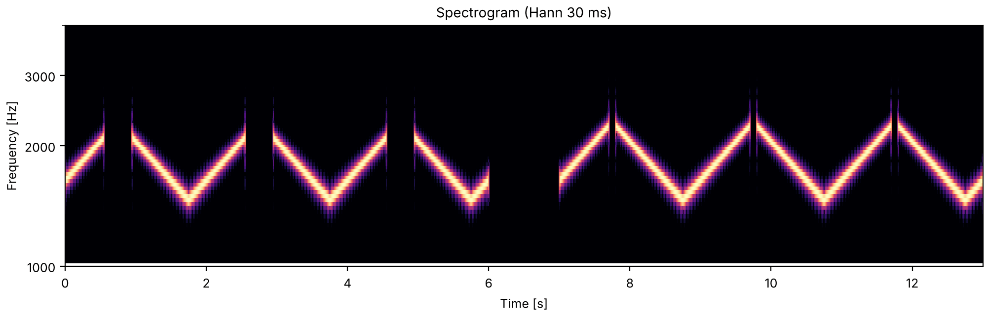
The top cut out, silent

Listen for the highest pitch the glide reaches. The top of each cycle is cut out, first by a wide silent cut, then by a narrow one. The booklet points out that the glide reaches higher before the narrow cut, as the spectrogram shows. The next sound fills the same cuts with noise.

Bregman & Ahad, Demonstration 30, after Dannenbring (1976). The glide of Demonstration 29, cut only at its top, by 400 ms in the first three cycles and by 100 ms in the next three, as in the booklet. Ours: three cycles of each, and a pause of 1 s between them.

cc7_the_top_cut_out_silent.flac, 13.0 s, mono

Plots of the the top cut out, silent sound
Code
tops = 0.75 + np.arange(0, 6, 2)


def top_cut(width, noise):
    cuts = on(t, tops - width / 2, width)
    return so.Sound((1 - cuts) * glide_tone + cuts * noise, FS).ramp(10e-3)


narrow_band = so.gaussian_noise(6, FS, band=(1500, 3000), rng=np.random.default_rng(30)).data[: len(t), 0]
sound = finish(so.concat([top_cut(0.4, 0), so.silence(1.0, FS), top_cut(0.1, 0)]))
fig, playhead = show(sound, fmin=1000, fmax=4000)

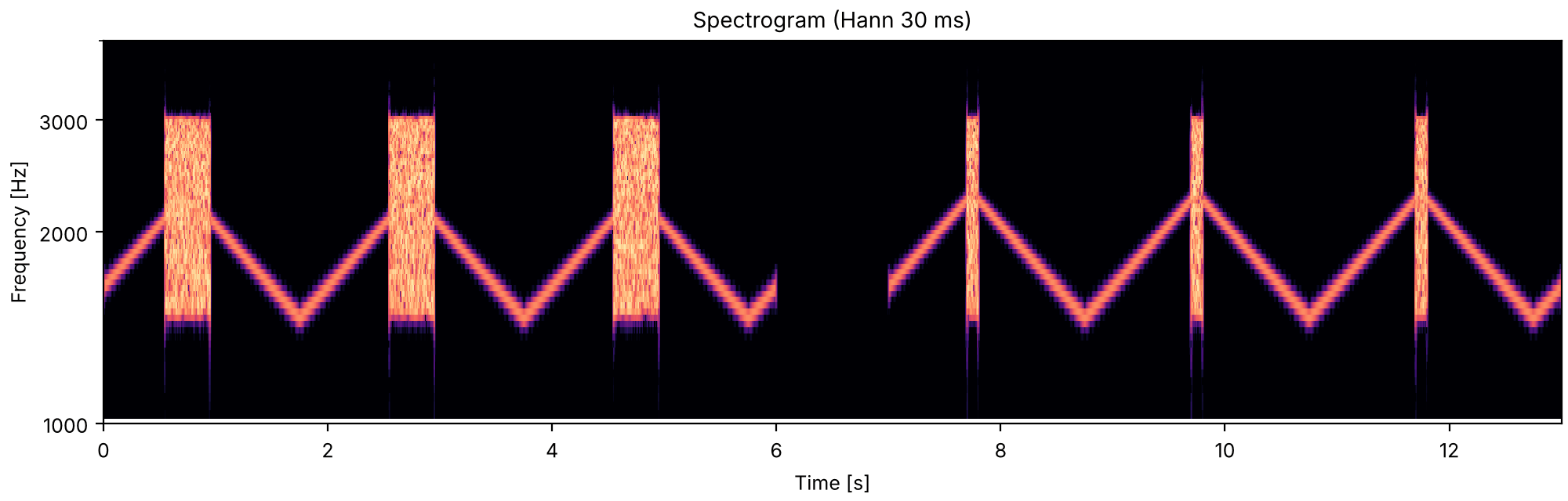
The top cut out, with noise

Listen for the highest pitch the glide seems to reach behind the noise, wide cut first and narrow cut second. If hearing carried each rise and fall on to where they would have met, both would seem to reach the same top. The booklet reports instead that the top seems higher with the narrow cut, and concludes that hearing joins the highest ends it actually heard rather than extrapolating them.

Bregman & Ahad, Demonstration 30, its second part: the same cuts filled with noise from 1500 to 3000 Hz, whose spectrum level the booklet gives as about 3 dB above the tone's. The booklet's Demonstration 28 says that white noise 20 times the tone's amplitude has the tone's spectrum level on its disc, which was sampled at 22255 Hz; taking that as the meaning of spectrum level, a 1500 Hz band 3 dB higher has an RMS about 10.4 times the tone's, the level used here. That reading is ours.

cc7b_the_top_cut_out_with_noise.flac, 13.0 s, mono

Plots of the the top cut out, with noise sound
Code
noise_rms = np.sqrt(2 * 20**2 * 1500 / (22255 / 2))
filler = noise_rms * narrow_band
sound = finish(so.concat([top_cut(0.4, filler), so.silence(1.0, FS), top_cut(0.1, filler)]))
fig, playhead = show(sound, fmin=1000, fmax=4000)

A sentence through a picket fence

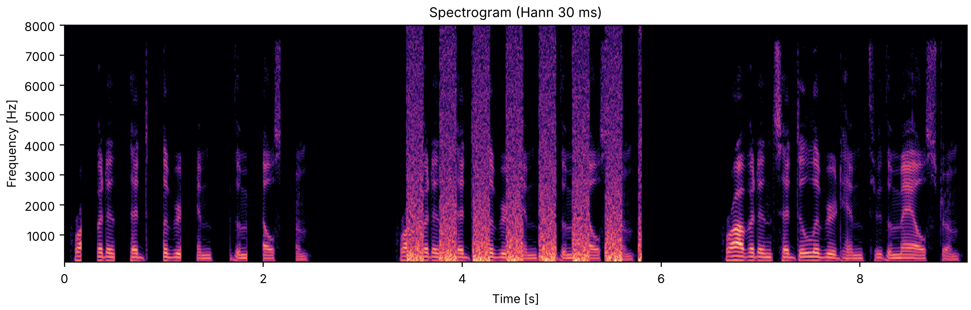
Listen for the sentence. Every other sixth of a second is cut out, first leaving silent gaps, then filled with loud noise; last comes the sentence intact. The booklet reports that with the noise the speech is heard as continuing behind it, though not always clearly, which it calls the picket-fence effect, after seeing an object as whole behind the pickets of a fence.

Bregman & Ahad, Demonstration 31, after Miller & Licklider (1950) and Warren (1982). A stand-in for its recording: the male talker's sentence used on the Fusion page (CMU ARCTIC, speaker bdl), where the disc has two sentences of its own. The speech is switched on and off abruptly by a 3 Hz square wave, so speech and gaps are each a sixth of a second; the noise is switched on and off abruptly to fill the gaps, falls 6 dB an octave, and has an RMS twice that of the loudest stretch of speech, all as in the booklet. The noise's band, 100 to 8000 Hz, is ours.

cc8_a_sentence_through_a_picket_fence.flac, 9.1 s, mono

Plots of the a sentence through a picket fence sound
Code
speech = so.load(fetch("docs/speech/bdl_arctic_a0131.flac"))
speech_t = speech.t
rng = np.random.default_rng(31)
tilted = so.gaussian_noise(speech.duration, speech.fs, band=(100, 8000), tilt=-6, rng=rng)


def picket_fence(rate):
    """The sentence with every other half-period of a `rate` Hz square wave cut out: silent
    gaps, then the same gaps filled with noise."""
    half = 0.5 / rate
    starts = np.arange(0, speech.duration, 2 * half)
    kept = on(speech_t, starts, half, ramp=0)
    segments = [speech.data[(speech_t >= start) & (speech_t < start + half), 0] for start in starts]
    loudest = max(np.sqrt(np.mean(segment**2)) for segment in segments)
    gapped = so.Sound(kept * speech.data[:, 0], speech.fs)
    filled = so.Sound(gapped.data[:, 0] + (1 - kept) * 2 * loudest * tilted.data[:, 0], speech.fs)
    return gapped, filled


pause = so.silence(0.75, speech.fs)
gapped, filled = picket_fence(3)
sound = finish(so.concat([gapped, pause, filled, pause, speech]))
fig, playhead = show(sound, fmin=100, fmax=8000, log=False)

Longer cuts in the sentence

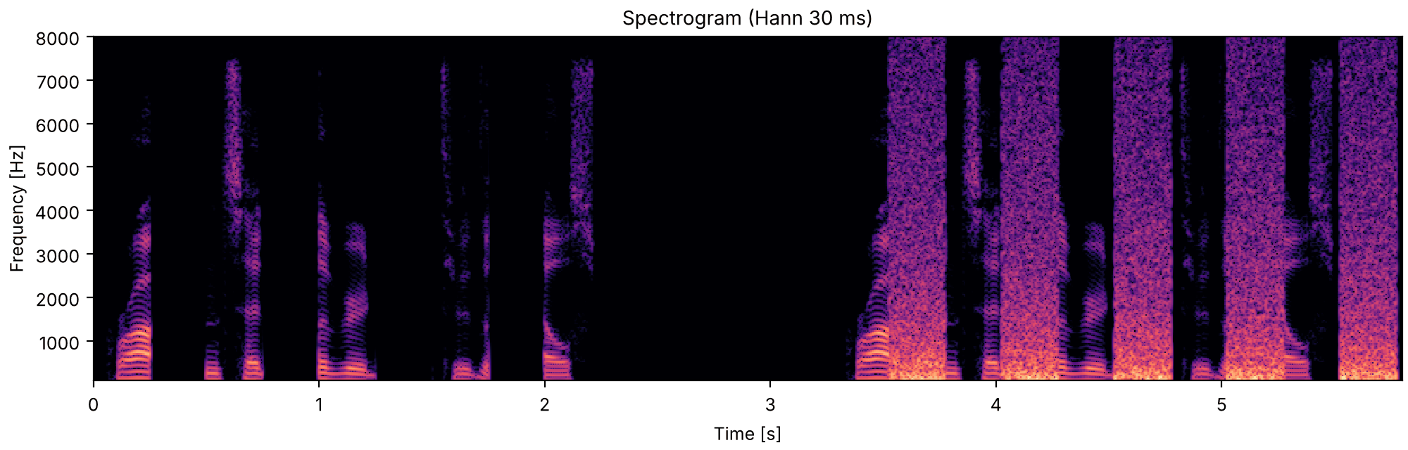
Listen for the same sentence with longer cuts, a quarter of a second each: silent gaps, then noise. The booklet reports that even with the longer cuts, listeners typically hear the speech as continuous behind the noise, though unclear.

Bregman & Ahad, Demonstration 31, its second example: a 2 Hz square wave, as in the booklet; otherwise built as the first.

cc8b_longer_cuts_in_the_sentence.flac, 5.8 s, mono

Plots of the longer cuts in the sentence sound
Code
gapped, filled = picket_fence(2)
sound = finish(so.concat([gapped, pause, filled]))
fig, playhead = show(sound, fmin=100, fmax=8000, log=False)

A noise swelling slowly, then suddenly

Listen for a hiss that swells and fades in each cycle at first. Then the swells become short and sudden, and the booklet reports a different sound: one long, steady hiss, briefly joined by a second, louder one. It calls this homophonic continuity: the soft noise is heard going on unchanged, and the extra energy of the sudden rise is heard as a new sound.

Bregman & Ahad, Demonstration 32, after Warren, Obusek & Ackroff (1972). White noise whose amplitude rests at 0.25 of its peak. In the gradual cycle, 744 ms in all, it holds for 120 ms, rises in a straight line to 1 in 252 ms, falls back in 252 ms and holds for 120 ms. In the sudden cycle, 724 ms in all, it holds for 342 ms, rises in 1 ms, stays at 1 for 32 ms, falls in 1 ms and holds for 348 ms; all as in the booklet. Ours: five cycles of each, and a pause of 1 s between them.

cc9_a_noise_swelling_slowly_then_suddenly.flac, 8.3 s, mono

Plots of the a noise swelling slowly, then suddenly sound
Code
def swells(knots, levels, n_cycles=5):
    period = knots[-1]
    t = np.arange(round(n_cycles * period * FS)) / FS
    noise = so.gaussian_noise(t[-1] + 1 / FS, FS, rng=np.random.default_rng(32)).data[: len(t), 0]
    return so.Sound(np.interp(t % period, knots, levels) * noise, FS).ramp(10e-3)


gradual = swells([0, 0.120, 0.372, 0.624, 0.744], [0.25, 0.25, 1, 0.25, 0.25])
sudden = swells([0, 0.342, 0.343, 0.375, 0.376, 0.724], [0.25, 0.25, 1, 1, 0.25, 0.25])
sound = finish(so.concat([gradual, so.silence(1.0, FS), sudden]))
fig, playhead = show(sound, fmin=100, fmax=10000)

What is left over

When the old sound is taken out of a mixture, what is left, the residual, is heard as a new sound of its own, even though nothing in the signal is shaped like it.

Two harmonics capturing their match

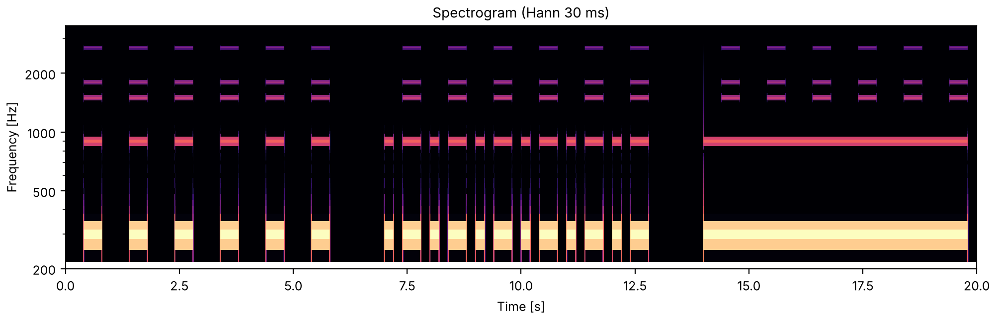
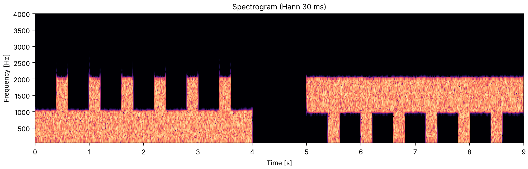
Listen for a rich low tone at first. Then it alternates with a thinner tone that holds only two of its harmonics, first with silences between them and then with none. The booklet reports that with the silences a second, higher tone is heard in the rich one only weakly, if at all, but without them it is heard clearly: the three harmonics the thinner tone does not have.

Bregman & Ahad, Demonstration 33. B, the rich tone, holds harmonics 1, 3, 5, 6 and 9 of 300 Hz at 0, -20, -28, -33 and -38 dB; A, the captor, holds harmonics 1 and 3 at the same levels. A cycle lasts 1 s: with silences, A for 200 ms, a 200 ms silence, B for 400 ms and another 200 ms silence; without, A for 600 ms and then B for 400 ms. First B alone, then the two alternations, as in the booklet. Ours: six cycles of each where the booklet plays eight, 10 ms ramps, and a pause of 1 s between the three. Here A and B are one sound whose harmonics 5, 6 and 9 switch on and off, so where A and B meet, harmonics 1 and 3 carry on unbroken.

cc10_two_harmonics_capturing_their_match.flac, 20.0 s, mono

Plots of the two harmonics capturing their match sound
Code
LEVELS_DB = {1: 0, 3: -20, 5: -28, 6: -33, 9: -38}
N_CYCLES = 6
B_ONSETS = np.arange(N_CYCLES) + 0.4  # in each 1 s cycle, B from 0.4 to 0.8 s
PART = N_CYCLES + 1.0
starts = {"B alone": 0.0, "with silences": PART, "no silences": 2 * PART}


def harmonics_on(t, n):
    """Harmonic `n`'s level over all three parts."""
    b = sum(on(t, start + B_ONSETS, 0.4, ramp=10e-3) for start in starts.values())
    if n not in (1, 3):
        return b
    a_with_silences = on(t, starts["with silences"] + B_ONSETS - 0.4, 0.2, ramp=10e-3)
    a_without = on(t, starts["no silences"] + B_ONSETS - 0.6, 0.6, ramp=10e-3)
    # the first A of the last part starts with the part, not 0.2 s before it
    return b + a_with_silences + a_without * (t >= starts["no silences"])


def residual_levels(t, f, n):
    return 10 ** (LEVELS_DB[n] / 20) * np.clip(harmonics_on(t, n), 0, 1)


sound = so.harmonic_complex(
    3 * PART - 1.0, FS, 300, harmonics=list(LEVELS_DB), amplitudes=residual_levels, phases="sine"
)
sound = finish(sound)
fig, playhead = show(sound, fmin=200, fmax=3500)

A wide band losing half to a narrow one

Listen for the short bursts of hiss between the long ones. A band of noise plays steadily while every 0.6 s a wider band, holding it and the band above it, sounds for a moment; then the same with the upper band steady. The booklet reports the steady band heard going on unbroken through each wide burst, which is heard as a short burst of the other band only: high in the first part, low in the second, although the wide bursts are the same in both.

Bregman & Ahad, Demonstration 34. B, the wide burst, holds 0 to 2 kHz and lasts 200 ms; L holds 0 to 1 kHz and H 1 to 2 kHz, and the one in play fills the 400 ms before and after each B, with no gaps, as in the booklet. Here the captor band runs on unbroken and the other half is switched on with it for each B, which makes B the full band at the same spectrum level. The booklet plays the two parts twice in alternation; this reproduction plays each once. Ours: six cycles of each, 5 ms cross-fades, and a pause of 1 s between them.

cc11_a_wide_band_losing_half_to_a_narrow_one.flac, 9.0 s, mono

Plots of the a wide band losing half to a narrow one sound
Code
def captured_band(captor, other, n_cycles=6):
    t = np.arange(round((0.6 * n_cycles + 0.4) * FS)) / FS
    gated = on(t, 0.4 + 0.6 * np.arange(n_cycles), 0.2)
    return so.Sound(captor.data[: len(t), 0] + gated * other.data[: len(t), 0], FS).ramp(10e-3)


low_half = so.gaussian_noise(4.0, FS, band=(0, 1000), rng=np.random.default_rng(34))
high_half = so.gaussian_noise(4.0, FS, band=(1000, 2000), rng=np.random.default_rng(35))
parts = [captured_band(low_half, high_half), so.silence(1.0, FS), captured_band(high_half, low_half)]
sound = finish(so.concat(parts))
fig, playhead = show(sound, fmin=50, fmax=4000, log=False)

Three bands in a cycle

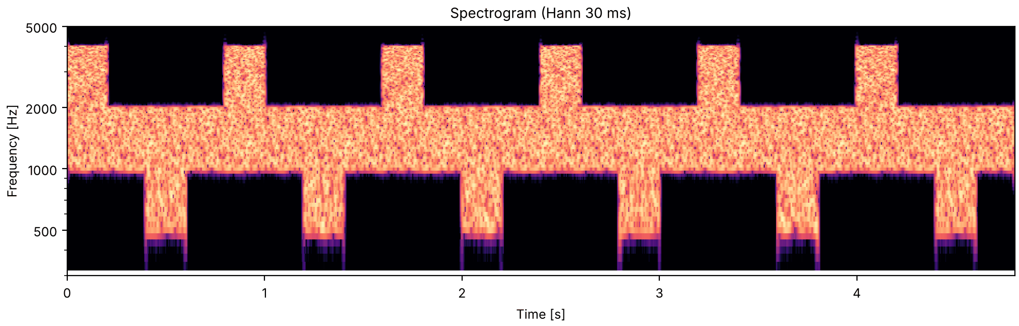
Listen for a busy pattern of hisses. Each cycle of 0.8 s is a high wide burst, a middle band, a low wide burst and the middle band again. The booklet describes the pattern as very complex at first; the three sounds that follow help to pick out three streams in it, which the booklet reports listeners can then hear without help: a high one, a low one and a middle band going on throughout.

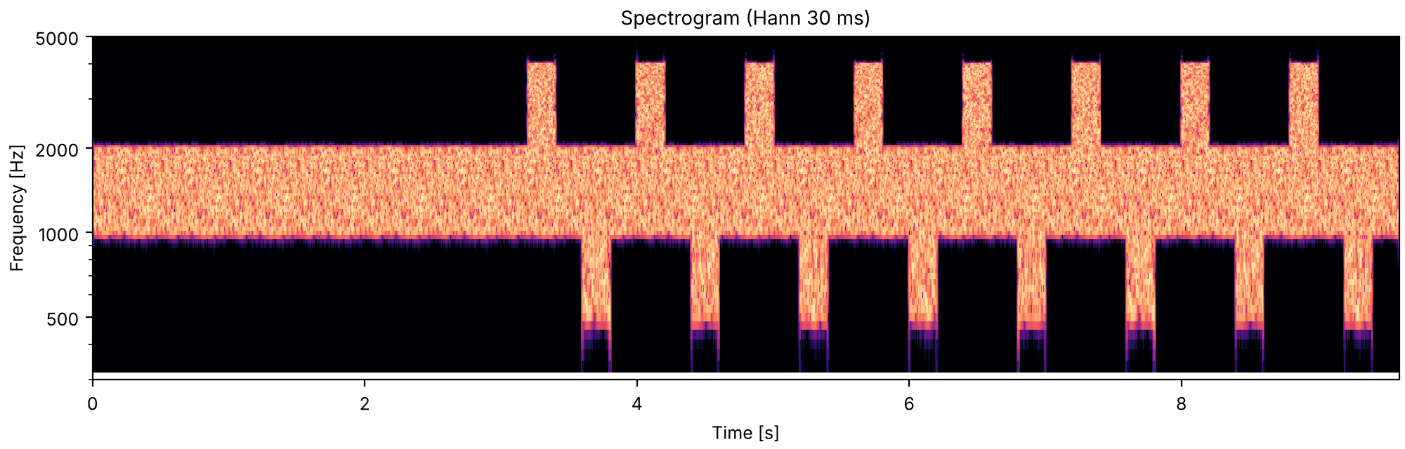
Bregman & Ahad, Demonstration 35. Three octave bands, L from 500 to 1000 Hz, M from 1000 to 2000 Hz and H from 2000 to 4000 Hz; A holds H and M, B holds L and M, and the cycle is A, M, B, M. As in the booklet, each band is a sum of equal tones in random phase on the harmonics of 2 Hz that fall in it, which gives sharp edges, and all three have the same spectrum level. The booklet does not give the bursts' length; 200 ms is ours. As on the previous example, the middle band runs on unbroken and the high and low bands are switched on with it, here with 5 ms cross-fades.

cc12_three_bands_in_a_cycle.flac, 4.8 s, mono

Plots of the three bands in a cycle sound
Code
def sharp_band(lo, hi, dur, seed):
    """Equal tones in random phase on the harmonics of 2 Hz from `lo` to `hi`: a band of noise
    with sharp edges. Each tone has RMS 1, so every such band has the same spectrum level."""
    harmonics = np.arange(lo // 2, hi // 2 + 1)
    rng = np.random.default_rng(seed)
    snd = so.harmonic_complex(dur, FS, 2, harmonics=harmonics, phases="random", rng=rng, ramp=0)
    return snd * np.sqrt(len(harmonics))


SLOT, LONGEST = 0.2, 9.6
L_BAND = sharp_band(500, 1000, LONGEST, seed=1)
M_BAND = sharp_band(1000, 2000, LONGEST, seed=2)
H_BAND = sharp_band(2000, 4000, LONGEST, seed=3)


def bands(standard=None, n_standard=0, n_full=6):
    """`n_standard` cycles with only the `standard` band ("L", "M" or "H"), then `n_full` of the
    whole pattern."""
    t = np.arange(round(4 * SLOT * (n_standard + n_full) * FS)) / FS
    full = 4 * SLOT * n_standard
    cycles = 4 * SLOT * np.arange(n_standard + n_full)
    before, after = cycles[cycles < full], cycles[cycles >= full]
    high = on(t, after, SLOT) + (standard == "H") * on(t, before, SLOT)
    low = on(t, after + 2 * SLOT, SLOT) + (standard == "L") * on(t, before + 2 * SLOT, SLOT)
    middle = on(t, [full], t[-1] + 1.0) + (standard == "M") * on(t, [0.0], full)
    mix = low * L_BAND.data[: len(t), 0] + middle * M_BAND.data[: len(t), 0] + high * H_BAND.data[: len(t), 0]
    return so.Sound(mix, FS)


sound = finish(bands())
fig, playhead = show(sound, fmin=300, fmax=5000)

Following the low band

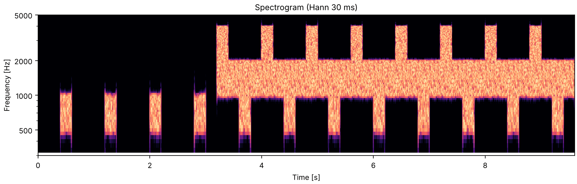
Listen for the low bursts that open this sound, alone, and keep following them once the full pattern starts. The booklet notes that for the first few cycles of the full pattern this can be hard, and that it gets easier as the cycles go on.

Bregman & Ahad, Demonstration 35, its first standard: four cycles of the low band alone, then eight of the full pattern. The number of cycles is ours.

cc12b_following_the_low_band.flac, 9.6 s, mono

Plots of the following the low band sound
Code
sound = finish(bands("L", 4, 8))
fig, playhead = show(sound, fmin=300, fmax=5000)

Following the high band

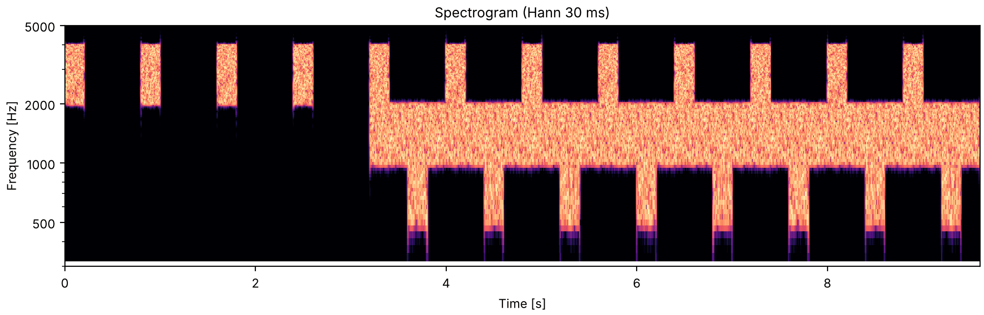
Listen for the high bursts, alone at first, then inside the full pattern. The booklet adds that the high band seems higher in the full pattern than alone.

Bregman & Ahad, Demonstration 35, its second standard, built as the first.

cc12c_following_the_high_band.flac, 9.6 s, mono

Plots of the following the high band sound
Code
sound = finish(bands("H", 4, 8))
fig, playhead = show(sound, fmin=300, fmax=5000)

Following the middle band

Listen for the steady middle band, alone at first, carrying on through the full pattern.

Bregman & Ahad, Demonstration 35, its third standard: the middle band steady for four cycles' time, then the full pattern.

cc12d_following_the_middle_band.flac, 9.6 s, mono

Plots of the following the middle band sound
Code
sound = finish(bands("M", 4, 8))
fig, playhead = show(sound, fmin=300, fmax=5000)

Glides and a vowel

The same capture with sounds that change: glides, where capture tells whether hearing takes the captured part as a continuation of what came before or as a repeat of it, and a vowel, which changes when one of its harmonics is captured.

A glide moving up to match another

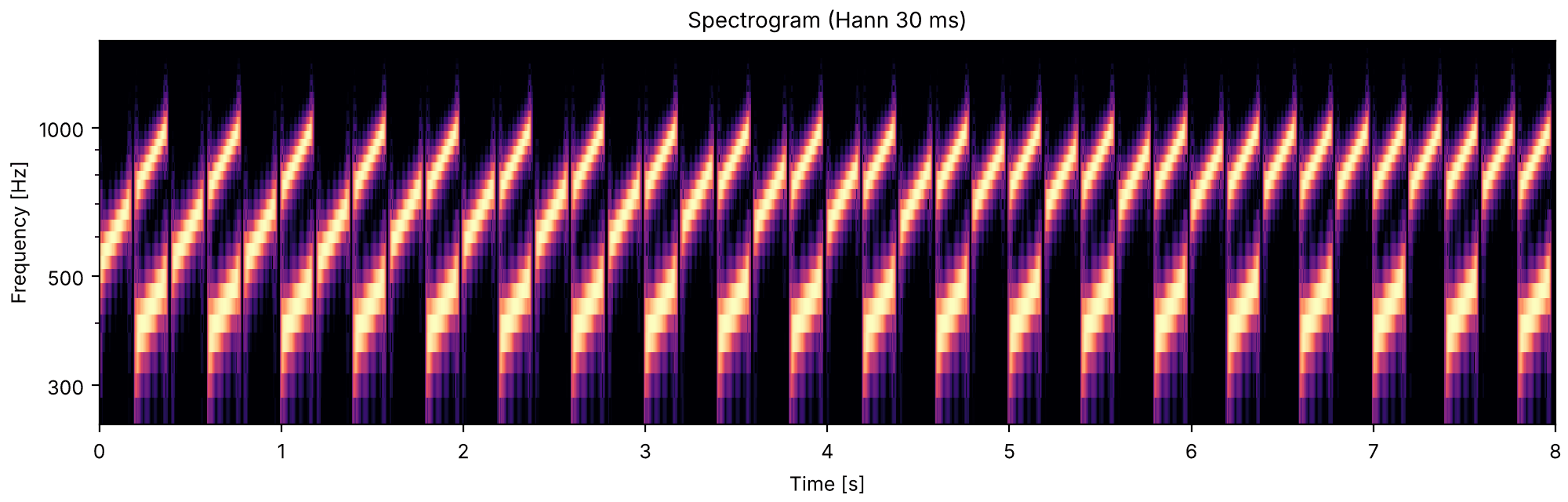
Listen for two high glides in a row, A and then B, with the lower glide C under B. When A captures B you hear high glides at twice the rate of the low one; when it does not, a pure A alternates with a richer B-and-C. A starts on B's path, half an octave below, and moves up in steps until it is the same glide as B. The booklet reports capture getting stronger as A approaches B, and best when B is a copy of A.

Bregman & Ahad, Demonstration 36. Pure glides rising at 2.5 octaves a second, 170 ms long, each followed by 30 ms of silence: B rises from 744 to 998 Hz and C, an octave below, from 372 to 499 Hz, always; A starts half an octave below B, where it lies on the same straight path, and ends the same as B, all as in the booklet. Ours: five positions of A (a step of an eighth of an octave), four cycles at each, played once where the booklet plays the series twice, equal levels, and 10 ms ramps.

cc13_a_glide_moving_up_to_match_another.flac, 8.0 s, mono

Plots of the a glide moving up to match another sound
Code
RATE, B_START, C_START = 2.5, 744, 372


def glides(a_start, n_cycles, gap=0.03, joined=False):
    """`n_cycles` of A, then B with C, each followed by `gap` seconds of silence; with `joined`, A
    and B are one glide with no silence between them."""
    period = 2 * (0.17 + gap)
    events = []
    for k in range(n_cycles):
        t = period * k
        if joined:
            events.append((t, glide(a_start, 0.17 + gap + 0.17, RATE)))
        else:
            events += [(t, glide(a_start, 0.17, RATE)), (t + 0.17 + gap, glide(B_START, 0.17, RATE))]
        events.append((t + 0.17 + gap, glide(C_START, 0.17, RATE)))
    return place(events, dur=period * n_cycles)


positions = B_START * 2 ** np.linspace(-0.5, 0, 5)
sound = finish(so.concat([glides(a, 4) for a in positions]))
fig, playhead = show(sound, fmin=250, fmax=1500)

A glide broken and unbroken

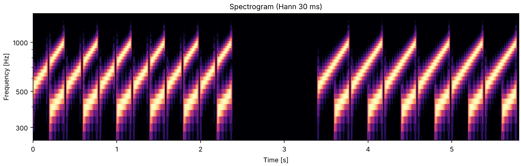
Listen for A and B as one long rising glide, broken by a short silence in the first part and unbroken in the second. The booklet reports that the long path is easier to follow with no silence, and concludes that for B to be heard as a continuation of A there should be no silent gap between them.

Bregman & Ahad, Demonstration 36, its second part: A on B's path, first with the 30 ms silence between them and then as one glide from A's start to B's end, as in the booklet. Ours: six cycles of each, played once where the booklet plays the part twice, and a pause of 1 s.

cc13b_a_glide_broken_and_unbroken.flac, 5.8 s, mono

Plots of the a glide broken and unbroken sound
Code
aligned = B_START / np.sqrt(2)
sound = finish(so.concat([glides(aligned, 6), so.silence(1.0, FS), glides(aligned, 6, joined=True)]))
fig, playhead = show(sound, fmin=250, fmax=1500)

Identical glides further and further apart

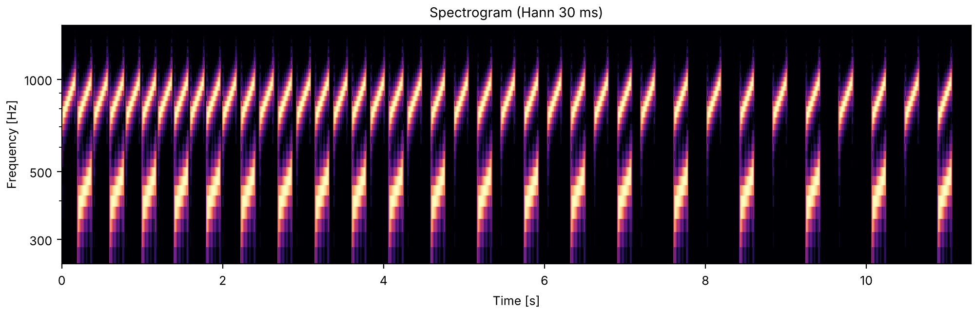
Listen for A and B as a repeated pair of identical high glides, while the silence after each glide grows in four steps. The booklet reports that the longer the silence, the harder it is to hear B as a repeat of A rather than as part of B-and-C.

Bregman & Ahad, Demonstration 36, its third part: A the same as B. The booklet does not give the silences; 30, 60, 120 and 240 ms after every glide, five cycles of each, are ours.

cc13c_identical_glides_further_and_further_apart.flac, 11.3 s, mono

Plots of the identical glides further and further apart sound
Code
sound = finish(so.concat([glides(B_START, 5, gap=gap) for gap in (0.03, 0.06, 0.12, 0.24)]))
fig, playhead = show(sound, fmin=250, fmax=1500)

A vowel losing part of a harmonic

Listen for the vowel. First four times as "i" (as in hid), then four times without its third harmonic, which the booklet hears as nasal, between "e" (bed) and "en" (bend). Then "i" eight more times, but with its third harmonic sounding on all the time, before, between and after the vowels. The booklet reports that the vowel then shifts toward "en": the steady tone is heard as a sound of its own, so part of the third harmonic is no longer counted in the vowel. It adds that the effect depends on the room, and is best heard over headphones.

Bregman & Ahad, Demonstration 37, after Darwin (1984). A vowel of harmonics of 125 Hz in sine phase, 450 ms long including 50 ms rise and decay, once a second; spectral peaks at 375, 2000, 2500 and 3500 Hz, all as in the booklet. The booklet set the harmonics' levels by ear and does not list them; here they come from four resonances at those peaks, with bandwidths 60, 100, 120 and 175 Hz, on a source falling 6 dB an octave, up to 4000 Hz, and are ours. The booklet's last part, comparisons with the third harmonic turned down by 3 to 18 dB, is left out; the pause of 1 s before the third part, and the third harmonic starting 0.5 s before it, are ours.

cc14_a_vowel_losing_part_of_a_harmonic.flac, 17.2 s, mono

Plots of the a vowel losing part of a harmonic sound
Code
PEAKS, BANDWIDTHS = (375, 2000, 2500, 3500), (60, 100, 120, 175)


def vowel_level(f):
    """Resonances at `PEAKS` (each 1 at 0 Hz) on a source falling 6 dB an octave."""
    gain = 1 / np.maximum(f, 1.0)
    for peak, bw in zip(PEAKS, BANDWIDTHS, strict=True):
        half = bw / 2
        below, above = (f - peak) ** 2 + half**2, (f + peak) ** 2 + half**2
        gain = gain * (peak**2 + half**2) / np.sqrt(below * above)
    return gain


i_onsets, en_onsets, captured_onsets = 0.25 + np.arange(4), 4.25 + np.arange(4), 9.25 + np.arange(8)


def vowel_gate(t, onsets):
    """The vowel's 450 ms with 50 ms rise and decay, at each of `onsets`."""
    return on(t, np.asarray(onsets) + 0.025, 0.4, ramp=0.05)


def vowel_harmonics(t, f, n):
    if n != 3:
        gate = vowel_gate(t, np.concatenate([i_onsets, en_onsets, captured_onsets]))
    else:
        gate = vowel_gate(t, i_onsets) + on(t, [8.75 + 0.025], 8.25 - 0.05, ramp=0.05)
    return vowel_level(f) * gate


harmonics = np.arange(1, 33)
sound = so.harmonic_complex(17.25, FS, 125, harmonics=harmonics, amplitudes=vowel_harmonics, phases="sine")
sound = finish(sound)
fig, playhead = show(sound, fmin=80, fmax=4500)

References

  • Bregman & Ahad (1996). Demonstrations of Auditory Scene Analysis: The Perceptual Organization of Sound (compact disc and booklet). Auditory Perception Laboratory, McGill University; MIT Press. Recordings and booklet.
  • Houtsma, Rossing & Wagenaars (1987). Auditory Demonstrations (compact disc and booklet). Institute for Perception Research (IPO), Eindhoven, and the Acoustical Society of America. Booklet.
  • Bregman (1990). Auditory Scene Analysis: The Perceptual Organization of Sound. MIT Press. doi:10.7551/mitpress/1486.001.0001.
  • Bregman & Tougas (1989). Propagation of constraints in auditory organization. Perception & Psychophysics 46(4), 395–396. doi:10.3758/BF03204994.
  • Dannenbring (1976). Perceived auditory continuity with alternately rising and falling frequency transitions. Canadian Journal of Psychology 30(2), 99–114. doi:10.1037/h0082053.
  • Darwin (1984). Perceiving vowels in the presence of another sound: constraints on formant perception. JASA 76(6), 1636–1647. doi:10.1121/1.391610.
  • Houtgast (1972). Psychophysical evidence for lateral inhibition in hearing. JASA 51(6B), 1885–1894. doi:10.1121/1.1913048.
  • Kominek & Black (2004). The CMU Arctic speech databases. Proc. 5th ISCA Speech Synthesis Workshop (SSW5), 223–224. ISCA Archive.
  • Miller & Licklider (1950). The intelligibility of interrupted speech. JASA 22(2), 167–173. doi:10.1121/1.1906584.
  • Warren (1982). Auditory Perception: A New Synthesis. Pergamon Press. Elsevier.
  • Warren, Obusek & Ackroff (1972). Auditory induction: perceptual synthesis of absent sounds. Science 176(4039), 1149–1151. doi:10.1126/science.176.4039.1149.

The papers were checked for their publication details only; the parameters on this page come from the booklets, and those marked as ours are choices made for this page.